Generalized Policy Iteration (GPI)

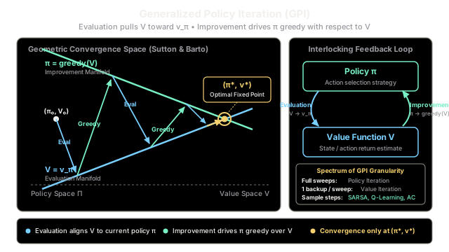
Generalized Policy Iteration (GPI) unifies reinforcement learning as a continuous interaction between policy evaluation and policy improvement, driving values and decisions toward mutual optimality.

Generalized Policy Iteration visualizes policy evaluation and greedy improvement as two interacting forces converging to the optimal policy and value function.

Why Does This Exist?

In reinforcement learning, finding an optimal policy presents a fundamental chicken-and-egg problem:

To evaluate how good a policy is ( $V \approx v_\pi$ ), you must fix the policy and measure its long-term return across every state.
To improve a policy ( $\pi \approx \arg\max_a Q(s, a)$ ), you need an accurate value function to guide your greedy action choices.

Classical Dynamic Programming resolves this dilemma through Policy Iteration, alternating between complete policy evaluation (iterating Bellman backups until $V$ converges to $v_\pi$ within machine precision) and complete policy improvement. While mathematically elegant, waiting for evaluation to converge before making a single policy tweak is computationally prohibitive for large state spaces, and completely impossible in real-time, sample-based learning.

Richard Sutton and Andrew Barto coined the term Generalized Policy Iteration (GPI) to capture the universal pattern operating underneath almost all reinforcement learning methods. GPI reveals that policy evaluation and policy improvement do not need to operate as exhaustive, serialized phases. Instead, they can interleave at any level of granularity—down to a single Bellman backup, an asynchronous state update, or a single sampled transition tuple $(s, a, r, s')$ .

Without the conceptual foundation of GPI, algorithms like Value Iteration, SARSA, Q-learning, and Actor-Critic appear as isolated heuristics. GPI establishes that all these methods are simply different trade-offs along a single continuum of update granularity, all converging to the exact same fixed point: the optimal policy $\pi^*$ and optimal value function $v_*$ .

Think of It Like This

Two legs walking forward

Imagine a hiker navigating rugged terrain toward a distant mountain peak.

Your left leg represents policy evaluation: it steps forward and plants firmly on the ground, measuring the exact elevation and stability of where your current strategy leads.

Your right leg represents policy improvement: once the left foot provides a stable reference, the right leg swings forward toward the steepest upward incline, steering your body toward a better heading.

Neither leg can reach the destination by itself. If the left leg took fifty steps without the right leg moving, you would merely stand in place, repeatedly recalibrating your measurement of the ground beneath you without making forward progress. Conversely, if your right leg tried to run forward without the left leg planting to measure the ground, you would blindly stumble off a cliff.

By alternating steps—plant the left foot to evaluate, swing the right foot to improve—both legs cooperate to propel you up the mountain.

Where the analogy stops: A hiker takes alternating steps of roughly equal length. In reinforcement learning, the "steps" can be completely asymmetrical. You might take ten evaluation sweeps for every improvement step, or you might take a single fractional gradient step on value and policy simultaneously, as in modern Actor-Critic architectures.

How It Actually Works

The Interplay of Evaluation and Improvement

GPI formalizes reinforcement learning as the ongoing interaction between two distinct operations defined on the joint space of policies $\Pi$ and value functions $\mathcal{V}$ :

Policy Evaluation ( $V \to v_\pi$ ): Holding the policy $\pi$ fixed, update the value function $V$ so that it more accurately reflects the expected return under $\pi$ . Under the Bellman expectation operator $T^\pi$ , the value of each state $s \in \mathcal{S}$ is pulled toward:
$v_\pi(s) = \sum_{a \in \mathcal{A}} \pi(a|s) \sum_{s' \in \mathcal{S}} \sum_{r} p(s', r | s, a) \left[ r + \gamma v_\pi(s') \right]$
where $\gamma \in [0, 1)$ is the discount factor and $p(s', r | s, a)$ denotes the transition probability.
Policy Improvement ( $\pi \to \text{greedy}(V)$ ): Holding the current value estimate $V$ fixed, update the policy $\pi$ to act greedily with respect to the action values induced by $V$ :
$\pi'(s) = \arg\max_{a \in \mathcal{A}} \sum_{s' \in \mathcal{S}} \sum_{r} p(s', r | s, a) \left[ r + \gamma V(s') \right]$
According to the Policy Improvement Theorem, if $q_\pi(s, \pi'(s)) \ge v_\pi(s)$ for all states $s$ , then the new policy $\pi'$ is guaranteed to achieve equal or greater return from every state: $v_{\pi'}(s) \ge v_\pi(s)$ .

Geometric Tug-of-War and the Universal Fixed Point

In the geometric phase space spanned by all possible policies and value functions, we can visualize two intersecting manifolds:

The Evaluation Manifold $\mathcal{M}_{\text{eval}} = \{(\pi, V) \mid V = v_\pi\}$ : the set of points where the value function is an exact reflection of the current policy.
The Improvement Manifold $\mathcal{M}_{\text{imp}} = \{(\pi, V) \mid \pi = \text{greedy}(V)\}$ : the set of points where the policy is strictly greedy with respect to the current value function.

At any arbitrary starting pair $(\pi_0, V_0)$ , the system lies on neither manifold:

When policy evaluation moves $V$ toward $v_\pi$ , it alters the value landscape. The current policy $\pi$ is typically no longer greedy with respect to the new value function.
When policy improvement updates $\pi$ to be greedy with respect to $V$ , the existing value function $V$ is no longer the true return for the updated policy.

Each process constantly destabilizes the other, creating a moving target. However, because each evaluation step contracts value error (by the Banach fixed-point theorem for the Bellman operator) and each improvement step monotonically increases or maintains expected return, the alternating steps trace a converging zigzag trajectory.

The only point in the entire space where both forces simultaneously cease to push is the unique intersection where both conditions hold at once:

V = v_\pi \quad \text{and} \quad \pi = \text{greedy}(V)

This condition satisfies the Bellman Optimality Equation:

v_*(s) = \max_{a \in \mathcal{A}} \sum_{s', r} p(s', r | s, a) \left[ r + \gamma v_*(s') \right]

Thus, the mutual equilibrium point is none other than the global optimum $(\pi^*, v_*)$ .

The Spectrum of GPI Instantiations

Every major control algorithm in reinforcement learning occupies a specific point on the GPI spectrum:

Algorithm	Evaluation Granularity	Improvement Granularity	Mechanism
Policy Iteration	Infinite (until $\Delta < \epsilon$ )	Full greedy sweep over $\mathcal{S}$	Complete Bellman expectation sweeps followed by policy replacement
Value Iteration	1 Bellman sweep	1 greedy sweep (merged into backup)	Bellman optimality backup combining evaluation and improvement in one step
Asynchronous DP	1 state backup	1 state greedy update	Updates arbitrary subsets of states in any order
SARSA (TD Control)	1 sampled step: $Q(S, A) \leftarrow Q + \alpha \delta$	Continuous $\epsilon$ -greedy update	On-policy sample-based backups drive evaluation and behavior
Q-Learning	1 off-policy sample backup	Continuous $\epsilon$ -greedy action choice	Off-policy evaluation targets $\max_a Q(S', a)$ directly
Actor-Critic	Critic updates weights $w$ via TD error	Actor updates weights $\theta$ via policy gradient	Continuous function approximation where Critic evaluates and Actor improves

Worked numerical example

Consider a small two-state Markov Decision Process:

States: $\mathcal{S} = \{s_1, s_2\}$
Actions: $\mathcal{A} = \{a_1, a_2\}$
Discount Factor: $\gamma = 0.5$
Transitions and deterministic rewards:
- In $s_1$ : action $a_1$ transitions to $s_1$ with reward $r = 1.0$ ; action $a_2$ transitions to $s_2$ with reward $r = 3.0$ .
- In $s_2$ : action $a_1$ transitions to $s_1$ with reward $r = 0.0$ ; action $a_2$ transitions to $s_2$ with reward $r = 2.0$ .

Let us trace truncated GPI with 1-step evaluation sweeps (Value Iteration style) starting from the suboptimal policy $\pi_0 = [a_1, a_1]$ and initial value estimates $V_0 = [0.0, 0.0]$ .

Iteration 1

Partial Evaluation Step (1 sweep under $\pi_0$ ):
$V_1(s_1) = R(s_1, \pi_0(s_1)) + \gamma V_0(s_1) = 1.0 + 0.5(0.0) = 1.0$ $V_1(s_2) = R(s_2, \pi_0(s_2)) + \gamma V_0(s_1) = 0.0 + 0.5(0.0) = 0.0$
Updated value vector: $V_1 = [1.0, 0.0]$ .
Policy Improvement Step ( $\pi_1 = \arg\max_a Q(s, a; V_1)$ ):
- For state $s_1$ : $Q(s_1, a_1) = 1.0 + 0.5 \times V_1(s_1) = 1.0 + 0.5(1.0) = 1.5$ $Q(s_1, a_2) = 3.0 + 0.5 \times V_1(s_2) = 3.0 + 0.5(0.0) = 3.0$ $\arg\max_a Q(s_1, a) = a_2$ (action flips from $a_1$ to $a_2$ ).
- For state $s_2$ : $Q(s_2, a_1) = 0.0 + 0.5 \times V_1(s_1) = 0.0 + 0.5(1.0) = 0.5$ $Q(s_2, a_2) = 2.0 + 0.5 \times V_1(s_2) = 2.0 + 0.5(0.0) = 2.0$ $\arg\max_a Q(s_2, a) = a_2$ (action flips from $a_1$ to $a_2$ ).
Updated policy vector: $\pi_1 = [a_2, a_2]$ .

Iteration 2

Partial Evaluation Step (1 sweep under $\pi_1$ ):
$V_2(s_1) = R(s_1, a_2) + \gamma V_1(s_2) = 3.0 + 0.5(0.0) = 3.0$ $V_2(s_2) = R(s_2, a_2) + \gamma V_1(s_2) = 2.0 + 0.5(0.0) = 2.0$
Updated value vector: $V_2 = [3.0, 2.0]$ .
Policy Improvement Step ( $\pi_2 = \arg\max_a Q(s, a; V_2)$ ):
- For state $s_1$ : $Q(s_1, a_1) = 1.0 + 0.5(3.0) = 2.5$ $Q(s_1, a_2) = 3.0 + 0.5(2.0) = 4.0 \implies \arg\max = a_2$
- For state $s_2$ : $Q(s_2, a_1) = 0.0 + 0.5(3.0) = 1.5$ $Q(s_2, a_2) = 2.0 + 0.5(2.0) = 3.0 \implies \arg\max = a_2$
Updated policy vector: $\pi_2 = [a_2, a_2] = \pi_1$ . The policy is already stable and optimal!

Value Convergence to Fixed Point

Subsequent evaluation sweeps under $\pi^*(s_1) = a_2, \pi^*(s_2) = a_2$ refine the values toward the true analytical fixed point:

v_*(s_2) = 2.0 + 0.5 v_*(s_2) \implies 0.5 v_*(s_2) = 2.0 \implies v_*(s_2) = 4.0

v_*(s_1) = 3.0 + 0.5 v_*(s_2) = 3.0 + 0.5(4.0) = 5.0

With each subsequent evaluation sweep:

Sweep 3: $V_3 = [3.0 + 0.5(2.0), 2.0 + 0.5(2.0)] = [4.0, 3.0]$
Sweep 4: $V_4 = [3.0 + 0.5(3.0), 2.0 + 0.5(3.0)] = [4.5, 3.5]$
Sweep 5: $V_5 = [3.0 + 0.5(3.5), 2.0 + 0.5(3.5)] = [4.75, 3.75]$
As $k \to \infty$ : $V_k \to [5.0, 4.0] = v_*$ .

Despite using only one evaluation sweep per policy update, GPI discovered the exact optimal policy $\pi^*$ on the very first improvement step.

Code

The following self-contained implementation compares Exact Policy Iteration (exhaustive evaluation sweeps) against Truncated GPI ( $k$ evaluation sweeps per improvement step), demonstrating how both converge to identical policies and values while drastically altering computation overhead:

1from typing import Dict, List, Tuple2
3
4class DiscreteMDP:5    """Represents a finite Markov Decision Process."""6
7    def __init__(8        self,9        num_states: int,10        num_actions: int,11        transitions: Dict[Tuple[int, int], List[Tuple[float, int, float]]],12        gamma: float = 0.9,13    ) -> None:14        self.num_states = num_states15        self.num_actions = num_actions16        # transitions maps (state, action) -> list of (probability, next_state, reward)17        self.transitions = transitions18        self.gamma = gamma19
20
21def generalized_policy_iteration(22    mdp: DiscreteMDP,23    eval_sweeps_per_iter: int = 1,24    max_outer_iters: int = 100,25    eval_tol: float = 1e-6,26) -> Tuple[List[int], List[float], int, int]:27    """Executes Generalized Policy Iteration with configurable evaluation granularity.28
29    Args:30        mdp: The discrete MDP environment.31        eval_sweeps_per_iter: Number of Bellman evaluation sweeps before each greedy32                              improvement step (e.g., 1 for Value Iteration, 100 for Policy Iteration).33        max_outer_iters: Safety threshold on outer policy improvement rounds.34        eval_tol: Convergence criterion for value changes.35
36    Returns:37        Tuple of (converged_policy, converged_values, total_eval_sweeps, policy_changes).38    """39    V = [0.0] * mdp.num_states40    policy = [0] * mdp.num_states  # Initial policy: choose action 0 everywhere41
42    total_eval_sweeps = 043    policy_changes = 044
45    for outer_step in range(max_outer_iters):46        # 1. Policy Evaluation Phase: update V toward v_pi47        for _ in range(eval_sweeps_per_iter):48            delta = 0.049            V_new = list(V)50            for s in range(mdp.num_states):51                a = policy[s]52                # Bellman expectation equation backup: V(s) = sum p * (r + gamma * V(s'))53                expected_return = sum(54                    prob * (reward + mdp.gamma * V[next_s])55                    for prob, next_s, reward in mdp.transitions[(s, a)]56                )57                V_new[s] = expected_return58                delta = max(delta, abs(V_new[s] - V[s]))59
60            V = V_new61            total_eval_sweeps += 162            if delta < eval_tol:63                break64
65        # 2. Policy Improvement Phase: update policy greedily with respect to V66        policy_stable = True67        for s in range(mdp.num_states):68            q_values = [69                sum(70                    prob * (reward + mdp.gamma * V[next_s])71                    for prob, next_s, reward in mdp.transitions[(s, a)]72                )73                for a in range(mdp.num_actions)74            ]75
76            best_action = max(range(mdp.num_actions), key=lambda a: q_values[a])77            if best_action != policy[s]:78                policy[s] = best_action79                policy_stable = False80                policy_changes += 181
82        # Convergence: policy is invariant and value estimates are steady83        if policy_stable and delta < eval_tol:84            break85
86    rounded_values = [round(v, 4) for v in V]87    return policy, rounded_values, total_eval_sweeps, policy_changes88
89
90if __name__ == "__main__":91    # Two-state MDP matching the worked numerical example92    # State 0 (s1), State 1 (s2); Actions 0 (a1), 1 (a2)93    # Transitions: (s, a) -> [(prob, next_s, reward)]94    mdp_transitions = {95        (0, 0): [(1.0, 0, 1.0)],  # s1, a1 -> s1, r=1.096        (0, 1): [(1.0, 1, 3.0)],  # s1, a2 -> s2, r=3.097        (1, 0): [(1.0, 0, 0.0)],  # s2, a1 -> s1, r=0.098        (1, 1): [(1.0, 1, 2.0)],  # s2, a2 -> s2, r=2.099    }100    env = DiscreteMDP(num_states=2, num_actions=2, transitions=mdp_transitions, gamma=0.5)101
102    print("=== Comparing Granularities of Generalized Policy Iteration ===")103
104    # 1. Truncated GPI with 1-sweep evaluation (Value Iteration style)105    pi_vi, v_vi, sweeps_vi, changes_vi = generalized_policy_iteration(106        env, eval_sweeps_per_iter=1, eval_tol=1e-7107    )108    print("GPI (k=1, Value Iteration style):")109    print(f"  Converged Policy: {pi_vi} (0: a1, 1: a2)")110    print(f"  Converged Values: {v_vi}")111    print(f"  Total Eval Sweeps: {sweeps_vi}, Policy Updates: {changes_vi}\n")112
113    # 2. Truncated GPI with 3-sweep evaluation114    pi_k3, v_k3, sweeps_k3, changes_k3 = generalized_policy_iteration(115        env, eval_sweeps_per_iter=3, eval_tol=1e-7116    )117    print("GPI (k=3, Truncated style):")118    print(f"  Converged Policy: {pi_k3}")119    print(f"  Converged Values: {v_k3}")120    print(f"  Total Eval Sweeps: {sweeps_k3}, Policy Updates: {changes_k3}\n")121
122    # 3. Exact Policy Iteration (100 sweeps ceiling for deep convergence)123    pi_pi, v_pi, sweeps_pi, changes_pi = generalized_policy_iteration(124        env, eval_sweeps_per_iter=100, eval_tol=1e-7125    )126    print("GPI (k=100, Exact Policy Iteration style):")127    print(f"  Converged Policy: {pi_pi}")128    print(f"  Converged Values: {v_pi}")129    print(f"  Total Eval Sweeps: {sweeps_pi}, Policy Updates: {changes_pi}")

Expected Output

1=== Comparing Granularities of Generalized Policy Iteration ===2GPI (k=1, Value Iteration style):3  Converged Policy: [1, 1] (0: a1, 1: a2)4  Converged Values: [5.0, 4.0]5  Total Eval Sweeps: 27, Policy Updates: 26
7GPI (k=3, Truncated style):8  Converged Policy: [1, 1]9  Converged Values: [5.0, 4.0]10  Total Eval Sweeps: 28, Policy Updates: 211
12GPI (k=100, Exact Policy Iteration style):13  Converged Policy: [1, 1]14  Converged Values: [5.0, 4.0]15  Total Eval Sweeps: 50, Policy Updates: 2

Watch Out For

The Full-Evaluation Fallacy

A frequent trap for practitioners new to dynamic programming and reinforcement learning is believing that policy evaluation must run to strict numerical convergence before policy improvement is valid or safe.

In practice, spending substantial compute on high-precision evaluation of a suboptimal, transient policy is largely wasted. The policy improvement step will immediately invalidate those precise values anyway. Furthermore, partial evaluation (even a single backup) provides an accurate enough directional signal to identify greedy action improvements.

The Fix: Embrace truncated evaluation. In tabular settings, run Value Iteration (1 sweep) or modified policy iteration with small $k \in [3, 10]$ . In deep reinforcement learning, decouple target networks and use small critic update counts per actor update rather than training the critic to zero TD error at every step.

Exploration Starvation in Greedy Improvement

When policy improvement aggressively forces the policy to be strictly greedy with respect to incomplete, early value estimates, the agent can become prematurely deterministic.

If the agent only explores actions favored by early noisy values, other state-action transitions are never visited, preventing the evaluation process from ever correcting under-estimated values. The algorithm locks into a suboptimal policy basin because the evaluation process lacks sample coverage.

The Fix: Ensure continuous exploration during the improvement step. In tabular methods, use $\epsilon$ -greedy action selection or optimistic initial values. In deep policy methods, incorporate maximum entropy objectives (as in Soft Actor-Critic) or action noise to guarantee that policy improvement never collapses coverage before values converge.

The Quick Version

Generalized Policy Iteration (GPI) is the unifying conceptual framework describing the mutual interaction between policy evaluation ( $V \to v_\pi$ ) and policy improvement ( $\pi \to \text{greedy}(V)$ ).
Neither evaluation nor improvement needs to finish before the other begins; they can interleave at any granularity from full sweeps to single-transition updates.
Evaluation pulls value toward the current policy, while improvement steers the policy to be greedy over the current value, each destabilizing the other to form a converging geometric zigzag.
The unique mutual fixed point where both processes reach simultaneous equilibrium is the global optimum $(\pi^*, v_*)$ .
Classical Policy Iteration, Value Iteration, SARSA, Q-learning, and Actor-Critic are all concrete algorithmic implementations of GPI.