Policy Iteration
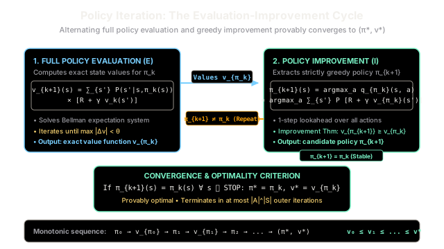
Policy iteration alternates between computing the exact value of the current policy and updating that policy to act greedily with respect to those values. Repeating this cycle guarantees reaching the strictly optimal policy in a finite number of iterations.
Why Does This Exist?
In a known Markov Decision Process (MDP), the goal is to discover an optimal policy that maximizes expected cumulative discounted returns. However, searching through all possible policies is a combinatorial nightmare: for a discrete MDP with state space and action space , there are distinct deterministic policies. In a simple grid with only 50 states and 4 movement directions, brute-force evaluation must inspect policies—a computational impossibility.
Evaluating an existing policy is a tractable linear problem, but finding the globally optimal policy directly is non-linear because choices made in one state dictate the values of upstream states. Without a systematic mechanism to navigate the space of policies, algorithms either stall in local heuristics or resort to intractable brute-force enumeration.
Policy iteration, introduced by Ronald Howard in 1960, solves this by decomposing control into two alternating sub-problems:
- Policy Evaluation: Compute the exact long-term value function for the agent's current policy .
- Policy Improvement: Construct an improved policy by acting greedily with respect to the freshly calculated value landscape .
The mathematical engine powering this loop is the Policy Improvement Theorem. It guarantees that each greedy update produces a policy that is strictly better than the previous one across all states, or identical if the policy is already globally optimal. Because finite MDPs possess a finite number of policies and no policy can ever repeat, policy iteration provably terminates at the exact globally optimal policy in a finite number of iterations.
Think of It Like This
Drafting and polishing an encyclopedia manuscript
Imagine an author collaborating with an editorial committee to produce a definitive technical handbook:
- Full Evaluation (The Comprehensive Editorial Audit): The author begins with a rough initial outline (). Before suggesting revisions, the editors read the entire manuscript from cover to cover. They calculate the exact pedagogical impact and clarity score of every single section under the current text (evaluating to absolute convergence).
- Policy Improvement (Targeted Chapter Revisions): With the complete scorecard in hand, the author inspects each chapter one by one. Whenever an alternative explanation or better case study yields a higher expected reader score based on the editorial audit, the author greedily substitutes that chapter's text (forming a revised draft ).
The author hands draft back to the committee. Because every substituted chapter was chosen based on exact evaluations, the Policy Improvement Theorem guarantees that draft is at least as good as, and typically much stronger than, draft . When the editors complete an audit and cannot find a single chapter revision that yields a higher score (), the handbook has reached its optimal version.
Where the analogy stops: Human writing involves subjective taste, stylistic ambiguity, and diminishing author stamina. In an MDP with discount factor , mathematical evaluation is strictly objective, monotonic, and mathematically bound to terminate at the unique global optimum without getting trapped in cyclical edits.
How It Actually Works
The Evaluation-Improvement Loop and Convergence Guarantees
Policy iteration alternates between two foundational operators in a closed loop:
1. Policy Evaluation ()
Given a policy , policy evaluation calculates the expected return for every state . The value function satisfies the linear Bellman expectation equation:
For deterministic policies where selects a single action:
This forms a system of linear equations with unknowns. It can be solved either directly in matrix form via , or iteratively through successive relaxation sweeps:
The sweeps repeat until , where is a small positive convergence threshold.
2. Policy Improvement ()
Once the exact value function is known, the agent evaluates the action-value function for every possible action :
The new policy is extracted greedily by choosing the action that maximizes this one-step lookahead:
If multiple actions tie for the maximum, the agent may pick any maximizing action deterministically or split selection probability equally.
3. The Policy Improvement Theorem and Finite Convergence
The theoretical backbone of the algorithm is the Policy Improvement Theorem: If for all , then:
If the inequality is strict in at least one state, the entire policy is strictly superior. If no action change occurs—meaning across all states—the policy is stable. At this point, the greedy action selection satisfies:
This is the Bellman Optimality Equation. Therefore, and .
Because an MDP with finite state space and finite action space has at most unique deterministic policies, and each iteration strictly increases the value function unless already optimal, no policy can ever be evaluated twice. Consequently, policy iteration is guaranteed to terminate in at most outer iterations. In practice, it converges in a tiny fraction of that bound (often fewer than 10 iterations even on complex problems).
Worked numerical example
Consider a 3-state chain MDP:
- States: . State is a terminal absorbing state with fixed value .
- Actions: .
- Discount factor: .
- Transition Dynamics & Rewards:
- In : action loops back to with reward . Action moves to with reward .
- In : action moves to with reward . Action transitions to terminal with reward .
- In terminal : absorbing state, all actions yield reward 0.
Cycle 0: Initial Policy
We initialize an arbitrary policy choosing everywhere:
Step 0.1: Policy Evaluation of Set up the Bellman expectation equations:
Step 0.2: Policy Improvement on Evaluate action-values :
-
For state :
-
For state :
Policy changed from to . Policy is not stable. Proceed to Cycle 1.
Cycle 1: Policy
Step 1.1: Policy Evaluation of Evaluate values under the newly proposed policy:
- In : action transitions to terminal :
- In : action transitions to :
Notice the monotonic value surge: and .
Step 1.2: Policy Improvement on Re-compute action-values using the new value landscape:
-
For state :
-
For state :
Updated policy . Because for all states, the policy is stable. The algorithm terminates.
Final Optimal Solution:
- Optimal Policy:
- Optimal Values:
Code
from typing import Dict, List, Tuple
# Type aliases representing discrete MDP components# State -> Action -> list of (transition_probability, next_state, immediate_reward)MDPTransitions = Dict[str, Dict[str, List[Tuple[float, str, float]]]]Policy = Dict[str, str]ValueFunction = Dict[str, float]
def policy_evaluation( policy: Policy, transitions: MDPTransitions, gamma: float = 0.5, theta: float = 1e-9,) -> ValueFunction: """Computes exact state values V_pi for a deterministic policy via Bellman sweeps.
Args: policy: Mapping of each state to its selected action. transitions: MDP transition dynamics and reward mapping. gamma: Discount factor in range [0, 1). theta: Convergence threshold for stopping iterative sweeps.
Returns: Converged state-value function mapping each state to its expected return. """ states = list(transitions.keys()) V: ValueFunction = {s: 0.0 for s in states}
while True: delta = 0.0 for s in states: chosen_action = policy[s] # Bellman expectation equation: # V(s) = sum_{s'} P(s'|s, a) * [R(s, a, s') + gamma * V(s')] expected_val = sum( prob * (reward + gamma * V[next_s]) for prob, next_s, reward in transitions[s][chosen_action] ) delta = max(delta, abs(expected_val - V[s])) V[s] = expected_val
if delta < theta: break
return V
def policy_improvement( V: ValueFunction, transitions: MDPTransitions, current_policy: Policy, gamma: float = 0.5,) -> Tuple[Policy, bool]: """Greedily extracts a new policy with respect to the value function V.
Args: V: Evaluated state values. transitions: MDP transition dynamics and reward mapping. current_policy: The policy that generated V. gamma: Discount factor in range [0, 1).
Returns: A tuple of (new_policy, is_stable). """ new_policy: Policy = {} policy_stable = True
for s, available_actions in transitions.items(): q_values: Dict[str, float] = {}
for a, outcomes in available_actions.items(): # Action-value Q(s, a) lookahead q_values[a] = sum( prob * (reward + gamma * V[next_s]) for prob, next_s, reward in outcomes )
# Greedily choose action maximizing Q(s, a) best_action = max(q_values, key=lambda action: q_values[action]) new_policy[s] = best_action
if best_action != current_policy[s]: policy_stable = False
return new_policy, policy_stable
def policy_iteration( transitions: MDPTransitions, gamma: float = 0.5, theta: float = 1e-9,) -> Tuple[Policy, ValueFunction, int]: """Runs the full Policy Iteration algorithm until policy convergence.
Returns: A tuple of (optimal_policy, optimal_values, total_cycles). """ # Initialize with an arbitrary deterministic policy (first action in each state) policy: Policy = {s: list(transitions[s].keys())[0] for s in transitions} cycles = 0
while True: cycles += 1 # Step 1: Policy Evaluation V = policy_evaluation(policy, transitions, gamma, theta)
# Step 2: Policy Improvement new_policy, is_stable = policy_improvement(V, transitions, policy, gamma)
policy = new_policy if is_stable: break
return policy, V, cycles
if __name__ == "__main__": # 3-state chain MDP from the worked numerical example: # State s3 is absorbing (terminal) with 0 return. mdp: MDPTransitions = { "s1": { "L": [(1.0, "s1", 0.0)], "R": [(1.0, "s2", 1.0)], }, "s2": { "L": [(1.0, "s1", 0.0)], "R": [(1.0, "s3", 10.0)], }, "s3": { "L": [(1.0, "s3", 0.0)], "R": [(1.0, "s3", 0.0)], }, }
optimal_policy, optimal_values, num_cycles = policy_iteration(mdp, gamma=0.5)
print(f"Optimal Policy: s1 -> {optimal_policy['s1']}, s2 -> {optimal_policy['s2']}") print(f"Optimal Values: V(s1) = {optimal_values['s1']:.1f}, V(s2) = {optimal_values['s2']:.1f}") print(f"Cycles to Convergence: {num_cycles}")
# Expected output: # Optimal Policy: s1 -> R, s2 -> R # Optimal Values: V(s1) = 6.0, V(s2) = 10.0 # Cycles to Convergence: 2Watch Out For
Over-evaluating early, rapidly changing policies
The most common trap in exact policy iteration is computing policy evaluation to tight numerical tolerance () in early outer cycles.
Symptom: The algorithm spends 95% to 99% of its total execution time inside the inner evaluation loop solving for values of an unstable policy that will flip its actions in the very next greedy improvement pass. As state spaces grow, this manifests as extreme latency between policy updates.
Root cause: Full policy evaluation requires solving a system of linear equations of size , either via an direct matrix inversion or dozens of iterative Bellman expectation sweeps. In the early iterations, knowing the precise decimal values is redundant; all that matters for improvement is whether action scores higher than action .
The fix: Use Truncated Policy Evaluation (also known as Modified Policy Iteration). Cap the inner evaluation loop at a fixed number of sweeps (e.g., to iterations), or use an adaptive threshold that starts loose and tightens as fewer policy actions flip. In the extreme case of , this converges directly into Value Iteration.
The Quick Version
- Alternating engine: Policy iteration alternates between full policy evaluation () and greedy policy improvement ().
- Monotonic improvement: By the Policy Improvement Theorem, each greedy step guarantees across every state, eliminating regression.
- Finite convergence: Termination triggers when no action flips (), provably reaching the unique optimal policy in at most outer iterations.
- Computation tradeoff: Policy iteration makes dramatic policy improvements in very few outer cycles compared to value iteration, but incurs high per-cycle cost from inner evaluation loops.