Gradient Monte Carlo Algorithm

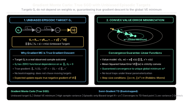
Gradient Monte Carlo updates parameterized value functions toward full-episode returns, achieving true gradient descent without bootstrapping bias.

Gradient Monte Carlo buffers full episodic trajectories to compute unbiased target returns, then updates parameter weights via true stochastic gradient descent.

Why Does This Exist?

When state spaces grow too large for lookup tables—such as continuous robotic joint spaces or high-dimensional board positions—reinforcement learning agents must approximate the state-value function using parameterized models, $\hat{v}(s, \mathbf{w}) \approx v_\pi(s)$ .

Tabular Monte Carlo simply averages observed returns per state. However, once function approximation is introduced, modifying the value of one state inevitably changes the values of neighboring states. To generalize correctly across unseen states, updates must minimize a formal global error metric, specifically the Mean Squared Value Error ( $\overline{\text{VE}}$ ).

Many function approximation methods rely on temporal-difference bootstrapping (such as Semi-Gradient TD), replacing future returns with the estimate $\hat{v}(S_{t+1}, \mathbf{w})$ . Because the bootstrap target itself depends on the parameter vector $\mathbf{w}$ , TD ignores the derivative of the target with respect to $\mathbf{w}$ . This turns TD into a semi-gradient method, stripping away conventional stochastic gradient descent (SGD) convergence guarantees.

Gradient Monte Carlo exists as the foundational baseline of true gradient methods in RL. By waiting until the episode terminates and using the complete empirical return $G_t$ as the target, the supervision signal is completely independent of the parameter vector $\mathbf{w}$ . Because $\mathbb{E}[G_t \mid S_t = s] = v_\pi(s)$ , every weight update follows the true negative gradient of the squared error in expectation, guaranteeing convergence to a global or local optimum.

Think of It Like This

End-of-Semester Student Evaluations

Imagine a university professor trying to evaluate and refine the clarity rating of each lecture module in a 15-week curriculum.

If the professor used bootstrapping (Temporal Difference learning), they would gauge the success of Lecture 3 by asking students how confident they feel about Lecture 4 immediately after Lecture 3 ends. If a student holds a misconception in Lecture 4, that biased self-assessment instantly corrupts the rating of Lecture 3.

Instead, Gradient Monte Carlo acts like comprehensive end-of-semester course evaluations and final exams. The professor delivers the entire syllabus from Week 1 through Week 15 without altering their baseline lecture ratings. Only after students complete their final cumulative exams does the professor inspect the total outcome ( $G_t$ ). If a student struggled on questions linked to concepts introduced in Lecture 3, the professor retroactively attributes that outcome and adjusts their teaching model's weights for those lecture topics.

Every final grade represents a concrete, uncorrupted realization of student comprehension. An individual student's exam score may fluctuate due to lack of sleep or personal distractions (high sample variance), but averaged across hundreds of students, the evaluation signal is completely unbiased.

Where the analogy stops: In reinforcement learning, the agent can adjust its decision policy across episodes based on these calibrated value weights, whereas a professor typically waits until the following academic year to modify their curriculum.

How It Actually Works

Mathematical Formulation and Objective Function

In on-policy value prediction with function approximation, we measure approximation quality using the Mean Squared Value Error, weighted by the on-policy state distribution $\mu(s)$ :

$\overline{\text{VE}}(\mathbf{w}) \doteq \sum_{s \in \mathcal{S}} \mu(s) \left[ v_\pi(s) - \hat{v}(s, \mathbf{w}) \right]^2$

Where:

$\mathbf{w} \in \mathbb{R}^d$ is the parameter weight vector.
$\hat{v}(s, \mathbf{w})$ is the differentiable parameterized value function approximation.
$\mu(s)$ is the fraction of time steps spent in state $s$ under policy $\pi$ ( $\sum_s \mu(s) = 1$ ).
$v_\pi(s)$ is the true underlying value of state $s$ .

To minimize $\overline{\text{VE}}(\mathbf{w})$ via stochastic gradient descent, the ideal parameter update for an observed state $S_t$ is proportional to the negative gradient of the squared error:

$\mathbf{w}_{t+1} \doteq \mathbf{w}_t - \frac{1}{2} \alpha \nabla_{\mathbf{w}} \left[ v_\pi(S_t) - \hat{v}(S_t, \mathbf{w}_t) \right]^2 = \mathbf{w}_t + \alpha \left[ v_\pi(S_t) - \hat{v}(S_t, \mathbf{w}_t) \right] \nabla \hat{v}(S_t, \mathbf{w}_t)$

In practice, the true value $v_\pi(S_t)$ is unknown. Gradient Monte Carlo substitutes the complete empirical discounted return $G_t$ for $v_\pi(S_t)$ :

$G_t \doteq \sum_{k=0}^{T - t - 1} \gamma^k R_{t+k+1}$

Yielding the Gradient Monte Carlo update rule:

$\mathbf{w}_{t+1} \doteq \mathbf{w}_t + \alpha \left[ G_t - \hat{v}(S_t, \mathbf{w}_t) \right] \nabla \hat{v}(S_t, \mathbf{w}_t)$

Where:

$\alpha > 0$ is the learning rate step-size parameter.
$\gamma \in [0, 1]$ is the discount factor.
$T$ is the terminal time step of the episode.
$\nabla \hat{v}(S_t, \mathbf{w}_t)$ is the column vector of partial derivatives with respect to the components of $\mathbf{w}_t$ .

Because $G_t$ is an unbiased estimator of $v_\pi(S_t)$ ( $\mathbb{E}[G_t \mid S_t] = v_\pi(S_t)$ ) and does not depend on $\mathbf{w}_t$ , the expected update vector is the exact negative gradient of $\overline{\text{VE}}(\mathbf{w})$ . Under standard Robbins-Monro step-size conditions ( $\sum \alpha_k = \infty, \sum \alpha_k^2 < \infty$ ), the algorithm is guaranteed to converge to a local optimum (and the unique global optimum under linear representations).

For linear function approximation, the value function is the inner product of the weight vector and a state feature vector $\mathbf{x}(s) \in \mathbb{R}^d$ :

$\hat{v}(s, \mathbf{w}) \doteq \mathbf{w}^\top \mathbf{x}(s) = \sum_{i=1}^d w_i x_i(s)$

The gradient reduces directly to the feature vector: $\nabla \hat{v}(s, \mathbf{w}) = \mathbf{x}(s)$ . The linear Gradient Monte Carlo update is:

$\mathbf{w}_{t+1} \doteq \mathbf{w}_t + \alpha \left[ G_t - \mathbf{w}_t^\top \mathbf{x}(S_t) \right] \mathbf{x}(S_t)$

Worked Numerical Example

Consider an episodic environment with 6 states, $\mathcal{S} = \{1, 2, 3, 4, 5, 6\}$ , partitioned into two coarse state-aggregation groups:

Group 1 ( $\{1, 2, 3\}$ ): represented by feature vector $\mathbf{x}(s) = [1.0, 0.0]^\top$ .
Group 2 ( $\{4, 5, 6\}$ ): represented by feature vector $\mathbf{x}(s) = [0.0, 1.0]^\top$ .

Parameters:

Learning rate: $\alpha = 0.5$
Discount factor: $\gamma = 1.0$ (undiscounted)
Initial weight vector: $\mathbf{w}_0 = [0.0, 0.0]^\top$

The agent generates an episode of length $T = 3$ :

$S_0 = 2$ (Group 1), takes action, receives reward $R_1 = 1.0$ , transitions to $S_1 = 4$ .
$S_1 = 4$ (Group 2), takes action, receives reward $R_2 = 0.0$ , transitions to $S_2 = 5$ .
$S_2 = 5$ (Group 2), takes action, receives reward $R_3 = 3.0$ , transitions to terminal state.

Step 1: Backward Return Computation

At episode termination, the agent computes returns recursively from $t = T-1$ down to $t = 0$ :

$G_2 = R_3 = 3.0$ $G_1 = R_2 + \gamma G_2 = 0.0 + (1.0)(3.0) = 3.0$ $G_0 = R_1 + \gamma G_1 = 1.0 + (1.0)(3.0) = 4.0$

Step 2: Sequential Weight Updates

Now the agent iterates through the trajectory to perform gradient updates.

Update for $t = 0$ ( $S_0 = 2 \in \text{Group 1}$ , $G_0 = 4.0$ ):

Feature vector: $\mathbf{x}(S_0) = [1.0, 0.0]^\top$
Prediction: $\hat{v}(S_0, \mathbf{w}_0) = [0.0, 0.0] \cdot [1.0, 0.0]^\top = 0.0$
Error: $\delta_0 = G_0 - \hat{v}(S_0, \mathbf{w}_0) = 4.0 - 0.0 = 4.0$
Gradient update: $\mathbf{w}_1 = \mathbf{w}_0 + \alpha \delta_0 \mathbf{x}(S_0) = \begin{bmatrix} 0.0 \\ 0.0 \end{bmatrix} + 0.5 \times 4.0 \times \begin{bmatrix} 1.0 \\ 0.0 \end{bmatrix} = \begin{bmatrix} 2.0 \\ 0.0 \end{bmatrix}$

Update for $t = 1$ ( $S_1 = 4 \in \text{Group 2}$ , $G_1 = 3.0$ ):

Feature vector: $\mathbf{x}(S_1) = [0.0, 1.0]^\top$
Prediction: $\hat{v}(S_1, \mathbf{w}_1) = [2.0, 0.0] \cdot [0.0, 1.0]^\top = 0.0$
Error: $\delta_1 = G_1 - \hat{v}(S_1, \mathbf{w}_1) = 3.0 - 0.0 = 3.0$
Gradient update: $\mathbf{w}_2 = \mathbf{w}_1 + \alpha \delta_1 \mathbf{x}(S_1) = \begin{bmatrix} 2.0 \\ 0.0 \end{bmatrix} + 0.5 \times 3.0 \times \begin{bmatrix} 0.0 \\ 1.0 \end{bmatrix} = \begin{bmatrix} 2.0 \\ 1.5 \end{bmatrix}$

Update for $t = 2$ ( $S_2 = 5 \in \text{Group 2}$ , $G_2 = 3.0$ ):

Feature vector: $\mathbf{x}(S_2) = [0.0, 1.0]^\top$
Prediction: $\hat{v}(S_2, \mathbf{w}_2) = [2.0, 1.5] \cdot [0.0, 1.0]^\top = 1.5$
Error: $\delta_2 = G_2 - \hat{v}(S_2, \mathbf{w}_2) = 3.0 - 1.5 = 1.5$
Gradient update: $\mathbf{w}_3 = \mathbf{w}_2 + \alpha \delta_2 \mathbf{x}(S_2) = \begin{bmatrix} 2.0 \\ 1.5 \end{bmatrix} + 0.5 \times 1.5 \times \begin{bmatrix} 0.0 \\ 1.0 \end{bmatrix} = \begin{bmatrix} 2.0 \\ 2.25 \end{bmatrix}$

Final Value Estimates after 1 Episode:

Group 1 states ( $\{1, 2, 3\}$ ): $\hat{v}(s, \mathbf{w}_3) = 2.0000$
Group 2 states ( $\{4, 5, 6\}$ ): $\hat{v}(s, \mathbf{w}_3) = 2.2500$

Notice how the second visit to Group 2 at $t = 2$ benefited from the update made at $t = 1$ , reducing the error from $3.0$ down to $1.5$ .

Code

1from typing import List, Tuple, Sequence2
3
4class LinearGradientMonteCarlo:5    """Gradient Monte Carlo for episodic value prediction with linear function approximation."""6
7    def __init__(self, num_features: int, alpha: float = 0.01, gamma: float = 1.0) -> None:8        self.num_features = num_features9        self.alpha = alpha10        self.gamma = gamma11        self.weights: List[float] = [0.0] * num_features12
13    def predict(self, features: Sequence[float]) -> float:14        """Compute estimated state value: v_hat(s, w) = w^T * x(s)."""15        return sum(w * x for w, x in zip(self.weights, features))16
17    def update_episode(18        self,19        trajectory: List[Tuple[Sequence[float], float]],20    ) -> List[float]:21        """Update weights using full-episode trajectory of (state_features, reward).22
23        Args:24            trajectory: List of (feature_vector, reward_received) pairs for t = 0 .. T-1.25        Returns:26            Updated weight vector.27        """28        if not trajectory:29            return list(self.weights)30
31        t_steps = len(trajectory)32        returns = [0.0] * t_steps33
34        # Backward pass: compute empirical return G_t = R_{t+1} + gamma * G_{t+1}35        running_g = 0.036        for t in reversed(range(t_steps)):37            reward = trajectory[t][1]38            running_g = reward + self.gamma * running_g39            returns[t] = running_g40
41        # Forward pass: stochastic gradient descent updates42        for t in range(t_steps):43            features = trajectory[t][0]44            target_g = returns[t]45            prediction = self.predict(features)46            error = target_g - prediction47
48            # Gradient for linear model is the feature vector x(s)49            for i in range(self.num_features):50                self.weights[i] += self.alpha * error * features[i]51
52        return list(self.weights)53
54
55# Demonstrate on the worked example56if __name__ == "__main__":57    # State aggregation: 2 feature dimensions (Group 1: [1, 0], Group 2: [0, 1])58    agent = LinearGradientMonteCarlo(num_features=2, alpha=0.5, gamma=1.0)59
60    # Trajectory:61    # S0=2 (Group 1) -> R1=1.0 -> S1=4 (Group 2) -> R2=0.0 -> S2=5 (Group 2) -> R3=3.0 -> Terminal62    episode_trajectory = [63        ([1.0, 0.0], 1.0),  # (features_S0, R1)64        ([0.0, 1.0], 0.0),  # (features_S1, R2)65        ([0.0, 1.0], 3.0),  # (features_S2, R3)66    ]67
68    final_weights = agent.update_episode(episode_trajectory)69
70    print(f"Final Weights: [w1={final_weights[0]:.4f}, w2={final_weights[1]:.4f}]")71    print(f"Value Estimate Group 1: {agent.predict([1.0, 0.0]):.4f}")72    print(f"Value Estimate Group 2: {agent.predict([0.0, 1.0]):.4f}")

1# Expected Output:2# Final Weights: [w1=2.0000, w2=2.2500]3# Value Estimate Group 1: 2.00004# Value Estimate Group 2: 2.2500

Watch Out For

High Variance and Episodic Horizon Latency

Because Gradient Monte Carlo constructs targets from un-bootstrapped sample trajectories, $G_t$ accumulates the stochastic transitions and reward noise across all future steps until termination:

$\operatorname{Var}[G_t] = \sum_{k=0}^{T-t-1} \gamma^{2k} \operatorname{Var}[R_{t+k+1} \mid S_t]$

In environments with long horizons or high action stochasticity, this variance causes updates to fluctuate wildly, requiring extremely small learning rates $\alpha$ and thousands of episodes to converge.

Furthermore, Gradient Monte Carlo cannot perform online updates during an ongoing episode. In tasks with very long or non-terminating (continuing) horizons ( $T \to \infty$ ), the algorithm is entirely unusable because $G_t$ cannot be computed.

The Fix: When sample efficiency or online adaptation is required, transition to n-step Semi-Gradient TD or eligibility traces ( $\text{TD}(\lambda)$ ). If retaining un-bootstrapped gradient guarantees is essential, apply variance-reduction techniques such as baseline subtraction, feature normalization, or learning rate schedules satisfying Robbins-Monro conditions.

The Quick Version

True Gradient Guarantee: Because complete returns $G_t$ do not depend on the parameter vector $\mathbf{w}$ , Gradient Monte Carlo follows the true negative gradient of the Mean Squared Value Error ( $\overline{\text{VE}}$ ).
Zero Bootstrapping Bias: Targets represent unbiased real-world trajectory returns, eliminating the self-referential estimation bias inherent to TD methods.
High Sample Variance: Accumulating stochastic rewards across entire trajectories introduces high variance, requiring smaller learning rates and more training episodes.
Strictly Episodic: Updates require trajectory completion and cannot be computed online mid-episode or applied to infinite-horizon continuing tasks.