Semi-Gradient TD(0)

Semi-gradient TD(0) updates value predictions by bootstrapping from the next state's estimate while treating that target as a fixed fact rather than backpropagating through it.

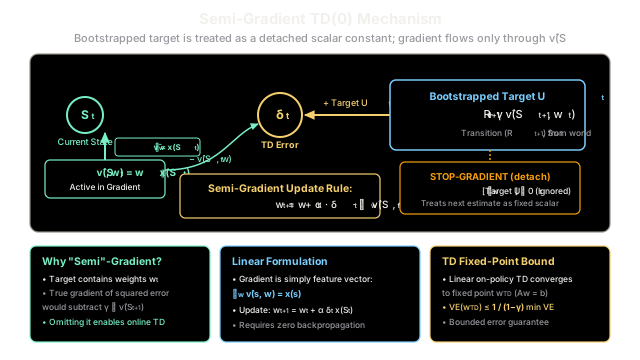
Why Does This Exist?

In supervised learning and Gradient Monte Carlo methods, optimization relies on true gradient descent: an agent observes an external, ground-truth label or complete episode return $G_t$ , computes the squared error loss $\frac{1}{2}[G_t - \hat{v}(S_t, \mathbf{w})]^2$ , and updates weights along the exact negative gradient $-\nabla_{\mathbf{w}} \mathcal{L}$ .

However, Monte Carlo updates cannot run online: they require waiting until an episode concludes to calculate $G_t$ , cannot function in non-terminating continuing tasks, and suffer from massive sample variance. To learn incrementally after every single transition $(S_t, R_{t+1}, S_{t+1})$ , Temporal Difference learning replaces the distant future return $G_t$ with a bootstrapped target:

$U_t = R_{t+1} + \gamma \hat{v}(S_{t+1}, \mathbf{w}_t)$

Here lies the mathematical dilemma: the target itself contains the parameter vector $\mathbf{w}_t$ .

If we applied standard calculus to differentiate the squared error $\frac{1}{2} [U_t(\mathbf{w}) - \hat{v}(S_t, \mathbf{w})]^2$ with respect to $\mathbf{w}$ , the gradient would backpropagate through both the current estimate and the target: $\nabla_{\mathbf{w}} \frac{1}{2} \left[ R_{t+1} + \gamma \hat{v}(S_{t+1}, \mathbf{w}) - \hat{v}(S_t, \mathbf{w}) \right]^2 = \delta_t \left[ \gamma \nabla_{\mathbf{w}} \hat{v}(S_{t+1}, \mathbf{w}) - \nabla_{\mathbf{w}} \hat{v}(S_t, \mathbf{w}) \right]$

Following this "full gradient" produces Residual Gradient algorithms, which converge painfully slowly, minimize the wrong objective (the Bellman error rather than the value error), and require double-sampling transitions.

Semi-gradient TD(0) resolves this dilemma with an intentional mathematical shortcut: it detaches the target. By treating the next-state estimate $\hat{v}(S_{t+1}, \mathbf{w}_t)$ as a fixed scalar constant during differentiation, semi-gradient TD(0) enables fast, efficient, online bootstrapping that converges reliably to a bounded fixed point under linear representations.

Think of It Like This

The Road Trip ETA Mileage Markers

Imagine you are driving across the country on a 500-mile highway road trip, continuously predicting your total travel time:

At Mile Marker 100: You look at your dashboard clock and current traffic conditions. Your internal model estimates your total travel time will be 8.0 hours.
At Mile Marker 110: Ten minutes later, you reach the next marker. You recalculate your expected total time from this new vantage point and realize it is now 8.3 hours (perhaps due to unexpected construction ahead).

To improve your prediction at Mile Marker 100, you compute the prediction error: $\text{Discrepancy} = 8.3\text{ hours} - 8.0\text{ hours} = +0.3\text{ hours}$

You immediately adjust your Mile Marker 100 prediction model upward to eliminate this 0.3-hour gap.

Crucially, when updating your estimate for Mile Marker 100, you treat the 8.3-hour estimate at Mile Marker 110 as an objective, frozen benchmark. You do not attempt to differentiate or second-guess how your future self at Marker 110 formulated that number; you simply treat it as an updated checkpoint and adjust your past prediction toward it.

Where the analogy stops: Human drivers know the physical laws of distance and speed. In reinforcement learning, the target estimate $\hat{v}(S_{t+1}, \mathbf{w})$ is itself a flawed, noisy hypothesis generated by the exact same parameter weights $\mathbf{w}$ that are being updated, meaning the target shifts continuously beneath the algorithm's feet as learning progresses.

How It Actually Works

Why Is It Called "Semi-Gradient"?

In general function approximation, let $\hat{v}(s, \mathbf{w})$ be a parameterized function with weight vector $\mathbf{w} \in \mathbb{R}^d$ .

If the target $U_t$ were an independent random variable uncorrelated with $\mathbf{w}_t$ , the gradient of the squared prediction error with respect to $\mathbf{w}$ would be:

$\nabla_{\mathbf{w}} \frac{1}{2} \left[ U_t - \hat{v}(S_t, \mathbf{w}) \right]^2 = - \left[ U_t - \hat{v}(S_t, \mathbf{w}) \right] \nabla_{\mathbf{w}} \hat{v}(S_t, \mathbf{w})$

In one-step TD, the target is $U_t = R_{t+1} + \gamma \hat{v}(S_{t+1}, \mathbf{w}_t)$ . Although this target explicitly depends on $\mathbf{w}_t$ , the semi-gradient method deliberately ignores the derivative of the target:

$\frac{\partial U_t}{\partial \mathbf{w}} \triangleq \mathbf{0} \quad (\text{treated as a detached constant})$

The parameter update rule is therefore:

$\mathbf{w}_{t+1} = \mathbf{w}_t + \alpha \underbrace{\left[ R_{t+1} + \gamma \hat{v}(S_{t+1}, \mathbf{w}_t) - \hat{v}(S_t, \mathbf{w}_t) \right]}_{\text{TD Error } \delta_t} \nabla_{\mathbf{w}} \hat{v}(S_t, \mathbf{w}_t)$

Because the update includes only the gradient of the estimated value $\hat{v}(S_t, \mathbf{w})$ and drops the gradient of the bootstrapped target, it is termed a semi-gradient method. In modern deep learning frameworks (PyTorch / JAX / TensorFlow), this detachment is implemented explicitly:

1# PyTorch equivalent of a semi-gradient TD target2td_target = reward + gamma * v_net(next_state).detach()

The Linear Semi-Gradient TD(0) Update

When using linear function approximation, state values are parameterized as an inner product:

$\hat{v}(s, \mathbf{w}) = \mathbf{w}^\top \mathbf{x}(s)$

Since $\nabla_{\mathbf{w}} \hat{v}(s, \mathbf{w}) = \mathbf{x}(s)$ , the semi-gradient update simplifies into a clean vector operation:

$\mathbf{w}_{t+1} = \mathbf{w}_t + \alpha \delta_t \mathbf{x}(S_t)$

where the scalar TD error is:

$\delta_t = R_{t+1} + \gamma \mathbf{w}_t^\top \mathbf{x}(S_{t+1}) - \mathbf{w}_t^\top \mathbf{x}(S_t)$

This update requires zero backpropagation, runs in $O(d)$ time, and performs linear feature projection online on every observed transition.

The TD Fixed Point and the Projection Matrix

Because semi-gradient TD(0) does not follow the true gradient of any fixed scalar loss function, it cannot be analyzed as ordinary gradient descent. Instead, it is an iterative projection operator: it repeatedly applies the Bellman operator $\mathcal{B}_\pi$ and projects the resulting values back onto the subspace representable by the linear feature matrix $\mathbf{X}$ .

Under on-policy state visitation distribution $\mu(s)$ , the expected weight update is:

$\mathbb{E}[\Delta \mathbf{w}_t] = \alpha \left( \mathbf{b} - \mathbf{A} \mathbf{w}_t \right)$

where:

$\mathbf{A} \triangleq \mathbb{E} \left[ \mathbf{x}(S_t) \left( \mathbf{x}(S_t) - \gamma \mathbf{x}(S_{t+1}) \right)^\top \right] \in \mathbb{R}^{d \times d}$
$\mathbf{b} \triangleq \mathbb{E} \left[ R_{t+1} \mathbf{x}(S_t) \right] \in \mathbb{R}^d$

When the step size $\alpha$ satisfies standard Robbins-Monro stochastic approximation conditions, linear semi-gradient TD(0) is guaranteed to converge to the unique TD fixed point $\mathbf{w}_{\text{TD}}$ :

$\mathbf{A} \mathbf{w}_{\text{TD}} = \mathbf{b} \implies \mathbf{w}_{\text{TD}} = \mathbf{A}^{-1} \mathbf{b}$

The matrix $\mathbf{A}$ is guaranteed to be positive definite whenever the feature covariance matrix has full rank and $\gamma < 1$ .

Furthermore, Tsitsiklis and Van Roy (1997) proved that the Mean Squared Value Error at this fixed point is strictly bounded:

$\overline{\text{VE}}(\mathbf{w}_{\text{TD}}) \le \frac{1}{1 - \gamma} \min_{\mathbf{w}} \overline{\text{VE}}(\mathbf{w})$

Even though semi-gradient TD does not follow the true error gradient, its asymptotic fixed point never diverges on-policy and remains tightly bounded near the best possible linear approximation.

Worked numerical example

Consider a 2-feature linear value approximator:

Current state $S_t$ with feature vector: $\mathbf{x}(S_t) = [1.0, 2.0]^\top$ .
Next state $S_{t+1}$ with feature vector: $\mathbf{x}(S_{t+1}) = [0.5, 1.0]^\top$ .
Current weight vector: $\mathbf{w}_t = [0.5, 1.0]^\top$ .
Observed transition reward: $R_{t+1} = 2.0$ .
Hyperparameters: discount factor $\gamma = 0.9$ , learning rate $\alpha = 0.1$ .

1. Forward Predictions

$\hat{v}(S_t, \mathbf{w}_t) = \mathbf{w}_t^\top \mathbf{x}(S_t) = (0.5 \times 1.0) + (1.0 \times 2.0) = 0.5 + 2.0 = \mathbf{2.500}$

$\hat{v}(S_{t+1}, \mathbf{w}_t) = \mathbf{w}_t^\top \mathbf{x}(S_{t+1}) = (0.5 \times 0.5) + (1.0 \times 1.0) = 0.25 + 1.0 = \mathbf{1.250}$

2. Bootstrapped Target Calculation

Treating $\hat{v}(S_{t+1}, \mathbf{w}_t)$ as a detached constant: $U_t = R_{t+1} + \gamma \hat{v}(S_{t+1}, \mathbf{w}_t) = 2.0 + 0.9 \times 1.250 = 2.0 + 1.125 = \mathbf{3.125}$

3. Temporal Difference Error

$\delta_t = U_t - \hat{v}(S_t, \mathbf{w}_t) = 3.125 - 2.500 = \mathbf{+0.625}$

4. Semi-Gradient Weight Update

The gradient with respect to $\mathbf{w}$ evaluates solely at the current state: $\nabla \hat{v}(S_t) = \mathbf{x}(S_t)$ : $\Delta \mathbf{w} = \alpha \delta_t \mathbf{x}(S_t) = 0.1 \times 0.625 \times \begin{bmatrix} 1.0 \\ 2.0 \end{bmatrix} = 0.0625 \times \begin{bmatrix} 1.0 \\ 2.0 \end{bmatrix} = \begin{bmatrix} 0.0625 \\ 0.1250 \end{bmatrix}$

$\mathbf{w}_{t+1} = \mathbf{w}_t + \Delta \mathbf{w} = \begin{bmatrix} 0.5 + 0.0625 \\ 1.0 + 0.1250 \end{bmatrix} = \begin{bmatrix} \mathbf{0.5625} \\ \mathbf{1.1250} \end{bmatrix}$

5. Verify Updated Current State Estimate

$\hat{v}(S_t, \mathbf{w}_{t+1}) = (0.5625 \times 1.0) + (1.1250 \times 2.0) = 0.5625 + 2.250 = \mathbf{2.8125}$

The prediction moved toward the target $3.125$ by exactly $\Delta \hat{v} = 0.3125$ , proportional to the step size and feature norm squared ( $\alpha \delta_t \|\mathbf{x}\|^2 = 0.0625 \times 5 = 0.3125$ ).

Code

1import math2from typing import List, Tuple3
4
5class LinearSemiGradientTD0:6    """Linear Semi-Gradient TD(0) for state-value prediction v_hat(s, w) = w^T x(s)."""7
8    def __init__(self, num_features: int, initial_weights: List[float]):9        assert len(initial_weights) == num_features10        self.num_features = num_features11        self.w = list(initial_weights)12
13    def predict(self, x: List[float]) -> float:14        """Compute inner product between weight vector and feature vector."""15        assert len(x) == self.num_features16        return sum(w_i * x_i for w_i, x_i in zip(self.w, x))17
18    def update(19        self,20        x_t: List[float],21        reward: float,22        x_next: List[float],23        gamma: float = 0.9,24        alpha: float = 0.1,25    ) -> Tuple[float, float, List[float]]:26        """Perform one-step semi-gradient TD(0) update.27
28        Returns:29            Tuple of (td_target, td_error, updated_weights).30        """31        # 1. Forward evaluations32        v_current = self.predict(x_t)33        # Detached next-state target: treated as fixed scalar constant34        v_next = self.predict(x_next)35
36        # 2. Compute bootstrapped TD target and error37        td_target = reward + gamma * v_next38        td_error = td_target - v_current39
40        # 3. Semi-gradient update: gradient is x_t (gradient of target is ignored)41        for i in range(self.num_features):42            self.w[i] += alpha * td_error * x_t[i]43
44        return td_target, td_error, list(self.w)45
46
47if __name__ == "__main__":48    # 2-feature numerical setup matching the worked example49    x_s = [1.0, 2.0]50    x_s_prime = [0.5, 1.0]51    w_initial = [0.5, 1.0]52    r_step = 2.053    discount = 0.954    step_size = 0.155
56    td_agent = LinearSemiGradientTD0(num_features=2, initial_weights=w_initial)57
58    # 1. Initial Predictions59    v_s_init = td_agent.predict(x_s)60    v_s_prime_init = td_agent.predict(x_s_prime)61    print("=== Linear Semi-Gradient TD(0) Verification ===")62    print(f"Initial v_hat(S_t):      {v_s_init:.4f}")63    print(f"Initial v_hat(S_t+1):    {v_s_prime_init:.4f}")64
65    assert math.isclose(v_s_init, 2.5), f"Expected 2.5, got {v_s_init}"66    assert math.isclose(67        v_s_prime_init, 1.2568    ), f"Expected 1.25, got {v_s_prime_init}"69
70    # 2. Semi-Gradient Transition Update71    target, error, updated_w = td_agent.update(72        x_t=x_s,73        reward=r_step,74        x_next=x_s_prime,75        gamma=discount,76        alpha=step_size,77    )78
79    print(f"\nBootstrapped TD Target: {target:.4f}")80    print(f"TD Error delta_t:       {error:.4f}")81    print(f"Updated Weight Vector:  {updated_w}")82
83    assert math.isclose(target, 3.125), f"Expected target 3.125, got {target}"84    assert math.isclose(error, 0.625), f"Expected error 0.625, got {error}"85    assert math.isclose(86        updated_w[0], 0.562587    ), f"Expected w[0] = 0.5625, got {updated_w[0]}"88    assert math.isclose(89        updated_w[1], 1.125090    ), f"Expected w[1] = 1.1250, got {updated_w[1]}"91
92    # 3. Verify Updated Current State Estimate93    v_s_updated = td_agent.predict(x_s)94    print(f"Updated v_hat(S_t):      {v_s_updated:.4f}")95    assert math.isclose(96        v_s_updated, 2.812597    ), f"Expected 2.8125, got {v_s_updated}"98
99    print(100        "\nAll semi-gradient mathematical update assertions passed successfully."101    )102
103# Expected Output:104# === Linear Semi-Gradient TD(0) Verification ===105# Initial v_hat(S_t):      2.5000106# Initial v_hat(S_t+1):    1.2500107#108# Bootstrapped TD Target: 3.1250109# TD Error delta_t:       0.6250110# Updated Weight Vector:  [0.5625, 1.125]111# Updated v_hat(S_t):      2.8125112#113# All semi-gradient mathematical update assertions passed successfully.

Watch Out For

Treating Semi-Gradient TD as True Gradient Descent & The Deadly Triad

Because the semi-gradient update formula looks superficially identical to standard gradient descent, practitioners often assume it is descending a well-behaved loss function. It is not.

Because the bootstrapped target changes continuously with the parameters, semi-gradient updates do not point along the negative gradient of any true scalar objective. In fact, when combined with the three elements of the Deadly Triad:

Function Approximation (linear or non-linear neural networks)
Bootstrapping (updating estimates from subsequent estimates, as in TD)
Off-Policy Training (evaluating target policy $\pi$ while collecting data with behavior policy $b$ )

Semi-gradient TD can diverge toward infinity, causing weight vectors to blow up and generating numerical NaN parameters (demonstrated by Baird's Counterexample).

The Fix:

Stay On-Policy When Bootstrapping: Linear semi-gradient TD(0) is mathematically guaranteed to converge if transitions are collected strictly on-policy.
Use True Gradient Off-Policy Algorithms: When off-policy learning is required with function approximation, use true gradient methods like Gradient TD (GTD2 / TDC) or Emphatic TD, which explicitly minimize the Projected Bellman Error (PBE) with dual-timescale updates.
Stabilize Deep Networks: In deep Q-learning (DQN), freeze the bootstrapped target using a separate periodic target network ( $\mathbf{w}^-$ ), temporarily transforming the semi-gradient update into an almost stationary supervised regression target.

The Quick Version

The semi-gradient shortcut: The bootstrapped target $R_{t+1} + \gamma \hat{v}(S_{t+1}, \mathbf{w})$ contains parameters $\mathbf{w}$ , but semi-gradient methods treat it as a detached constant ( $\nabla_{\mathbf{w}} \text{Target} \equiv \mathbf{0}$ ) during differentiation.
Linear update formula: With linear features, the gradient is simply the feature vector ( $\nabla \hat{v} = \mathbf{x}(s)$ ), simplifying updates to $\mathbf{w}_{t+1} = \mathbf{w}_t + \alpha \delta_t \mathbf{x}(S_t)$ without backpropagation.
The TD fixed point: Linear on-policy semi-gradient TD converges to a unique stationary point $\mathbf{w}_{\text{TD}} = \mathbf{A}^{-1}\mathbf{b}$ governed by an iterative Bellman projection operator.
Deadly Triad awareness: Because it is not true gradient descent, semi-gradient updating can diverge if paired with off-policy data and function approximation; on-policy linear training remains strictly stable.