Mean Field Multi-Agent RL

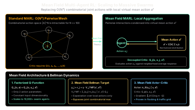
Instead of tracking thousands of individual neighbors, each agent coordinates against the average behavior of its local crowd.

Why Does This Exist?

In real-world multi-agent applications—such as metropolitan traffic flow, high-frequency financial order books, and drone swarm coordination—the number of participating agents $N$ easily scales into the hundreds or thousands ( $N \gg 100$ ).

Standard multi-agent reinforcement learning (MARL) paradigms break down catastrophically at this scale:

Centralized Critic Architectures (MADDPG): The centralized critic $Q(s, a_1, a_2, \dots, a_N)$ takes the concatenation of all agent actions as input. The input dimension scales as $\mathcal{O}(N)$ , and the joint action space grows combinatorially as $|\mathcal{A}|^N$ , creating an intractable optimization problem.
Value Factorization Methods (VDN, QMIX): While computationally more scalable, value decomposition requires mixing networks with monotonicity constraints. When coordinating hundreds of homogeneous agents, individual credit assignment becomes diluted and computationally prohibitive.
Independent Q-Learning (IQL): Ignores peer interactions entirely, causing rampant non-stationarity as thousands of agents update their policies simultaneously.

Mean Field Multi-Agent Reinforcement Learning (MF-MARL) (Yang et al., 2018) resolves this scalability barrier by borrowing a foundational concept from statistical physics: Mean Field Theory.

Instead of computing complex pairwise interactions between an agent and every other individual in the swarm, MF-MARL approximates all neighbor interactions through a single localized virtual mean action $\bar{a}^j$ . This reduces an intractable $\mathcal{O}(N^2)$ joint interaction network into an efficient $\mathcal{O}(N)$ local aggregation problem.

Think of It Like This

A sardine in a massive school of ten thousand fish

Imagine swimming as a single sardine inside a bait ball containing 10,000 fish fleeing from an apex predator.

The Standard MARL Approach (Pairwise Calculation): The sardine attempts to calculate the precise distance, swimming velocity, and turning angle of all 9,999 other individual fish simultaneously. Its tiny brain would overheat instantly under the computational load.
The Independent RL Approach: The sardine swims blindly, treating all other fish as passive water turbulence. It inevitably crashes into neighbors or gets separated from the protective school.
The Mean Field Approach: The sardine observes only the collective optical flow of the 5 or 6 fish immediately adjacent to it. It computes their average heading and velocity (the local mean field). If the local cluster veers 30 degrees to the left, the sardine veers 30 degrees to the left.

Because every fish executes this identical local mean-field alignment rule, coordinated swarm maneuvers—such as tight evasive vortices and shimmering flash expansions—ripple smoothly across the entire 10,000-fish school without requiring a central leader or individual-to-individual telepathy.

Where the analogy stops: Biological fish in a school share identical physical bodies, identical swimming dynamics, and symmetric objectives (survival). In real-world multi-agent engineering problems (such as electric vehicle grid charging or heterogeneous robot logistics), agents may have asymmetric battery capacities, different geographical goals, or specialized roles. In those cases, a naive spatial average can wash out critical individual distinctions unless augmented with graph attention.

How It Actually Works

Mean Action Approximation and the Mean Field Bellman Equation

Let an environment contain $N$ agents. For a given agent $j$ , let $\mathcal{N}(j)$ denote the set of neighboring agents within agent $j$ 's observation or communication radius.

1. The Virtual Mean Action

Each discrete action is represented as a one-hot vector $a_k \in \{0, 1\}^D$ , or a continuous action vector. Agent $j$ computes the local mean action $\bar{a}^j$ by averaging the action vectors across its neighborhood:

\bar{a}^j = \frac{1}{|\mathcal{N}(j)|} \sum_{k \in \mathcal{N}(j)} a_k

The mean action $\bar{a}^j \in [0, 1]^D$ represents the empirical probability distribution of neighbor behaviors.

2. Q-Function Factorization

In standard cooperative MARL, the centralized action-value function depends on the entire joint action profile $\mathbf{a} = (a_1, \dots, a_N)$ :

Q_j(s, \mathbf{a}) = Q_j(s, a_j, \mathbf{a}_{-j})

Using a first-order Taylor expansion around the local mean action $\bar{a}^j$ , Yang et al. (2018) proved that the joint Q-function can be factorized into a compact 2-argument function:

Q_j(s, \mathbf{a}) \approx Q_j(s, a_j, \bar{a}^j)

This reduces the action argument dimensionality from $N \times D$ to just $2 \times D$ , regardless of whether the swarm contains 10 agents or 100,000 agents.

3. Mean Field Q-Learning (MF-Q)

With the factorized Q-function, the Bellman target for agent $j$ simplifies from an intractable joint maximization into an expectation over its own local actions:

y_j = r_j + \gamma v_j^{\text{MF}}(s')

where the next-state mean field value function $v_j^{\text{MF}}(s')$ is computed as:

v_j^{\text{MF}}(s') = \sum_{a_j \in \mathcal{A}_j} \pi_j(a_j \mid s', \bar{a}'^j) \, Q_j(s', a_j, \bar{a}'^j)

The future mean action $\bar{a}'^j$ is estimated from the previous iteration's neighbor policies:

\bar{a}'^j = \frac{1}{|\mathcal{N}(j)|} \sum_{k \in \mathcal{N}(j)} \mathbb{E}_{a'_k \sim \pi_k(\cdot \mid s')} [a'_k]

4. Mean Field Actor-Critic (MF-AC)

For continuous action spaces or complex policies, each agent maintains a decentralized actor $\pi_{\theta_j}(a_j \mid s, \bar{a}^j)$ and updates its weights using policy gradient:

\nabla_{\theta_j} J(\theta_j) = \mathbb{E} \left[ \nabla_{\theta_j} \log \pi_{\theta_j}(a_j \mid s, \bar{a}^j) \, Q_{\phi_j}(s, a_j, \bar{a}^j) \right]

During execution, each agent only needs to estimate or observe the local average action $\bar{a}^j$ to select its optimal action $a_j$ .

Worked numerical example

Consider agent $j$ moving in a 2D grid swarm. The action space consists of 4 discrete movement directions: $\mathcal{A} = \{\text{Up (U)}, \text{Down (D)}, \text{Left (L)}, \text{Right (R)}\}$ encoded as 4D one-hot vectors $[U, D, L, R]$ .

1. Compute Local Mean Action

Agent $j$ has $|\mathcal{N}(j)| = 4$ immediate neighbors. In the current step, the neighbors take the following actions:

Neighbor 1: Up $\to a_1 = [1, 0, 0, 0]$
Neighbor 2: Up $\to a_2 = [1, 0, 0, 0]$
Neighbor 3: Down $\to a_3 = [0, 1, 0, 0]$
Neighbor 4: Left $\to a_4 = [0, 0, 1, 0]$

Summing the neighbor action vectors:

\sum_{k=1}^4 a_k = [1+1+0+0, \; 0+0+1+0, \; 0+0+0+1, \; 0+0+0+0] = [2, 1, 1, 0]

The local mean action vector is:

\bar{a}^j = \frac{1}{4} [2, 1, 1, 0] = [0.50, 0.25, 0.25, 0.00]

This vector indicates that $50\%$ of the neighborhood is moving Up, $25\%$ Down, and $25\%$ Left.

2. Evaluate Mean Field Q-Values

Given current state $s = 1.0$ and neighborhood mean action $\bar{a}^j = [0.50, 0.25, 0.25, 0.00]$ , agent $j$ 's neural Q-network evaluates the 4 candidate actions:

$Q_j(s, \text{U}, \bar{a}^j) = 4.20$ (aligns with flock heading)
$Q_j(s, \text{D}, \bar{a}^j) = 2.10$ (opposes flock heading)
$Q_j(s, \text{L}, \bar{a}^j) = 1.80$
$Q_j(s, \text{R}, \bar{a}^j) = 1.20$

Agent $j$ greedily selects action $a_j^* = \text{U}$ with predicted value $Q = 4.20$ .

3. Compute Bellman Target and TD Error

The environment executes the transition:

Immediate reward awarded: $r_j = 1.50$ .
Successor state: $s' = 1.20$ .
Next estimated neighbor mean action: $\bar{a}'^j = [0.60, 0.20, 0.20, 0.00]$ .
Discount factor: $\gamma = 0.90$ .
Estimated next-state value: $v_j^{\text{MF}}(s', \bar{a}'^j) = 4.50$ .

The Mean Field Bellman target is:

y_j = r_j + \gamma v_j^{\text{MF}}(s', \bar{a}'^j) = 1.50 + 0.90(4.50) = 1.50 + 4.05 = 5.55

The temporal difference (TD) error for updating $Q_j$ is:

\delta_j = y_j - Q_j(s, a_j^*, \bar{a}^j) = 5.55 - 4.20 = +1.35

Agent $j$ updates its weights via gradient descent on $\frac{1}{2} \delta_j^2$ with constant input complexity, regardless of how many thousands of agents populate the broader swarm.

Code

1from typing import Dict, List, Tuple2
3
4class MeanFieldMARLSimulator:5    """Demonstrates Mean Field Multi-Agent RL (MF-MARL; Yang et al., 2018):6
7    1. Aggregates neighbor one-hot actions into local mean action vector a_bar8    2. Evaluates Mean Field Q-values Q(s, a_j, a_bar^j)9    3. Calculates MF-Q Bellman target and TD error10    """11
12    def __init__(self, gamma: float = 0.90) -> None:13        self.gamma = gamma14
15    @staticmethod16    def compute_mean_action(neighbor_actions: List[List[float]]) -> List[float]:17        """Averages one-hot action vectors of neighboring agents in N(j):18
19        a_bar^j = (1 / |N(j)|) * sum_{k in N(j)} a_k20        """21        num_neighbors = len(neighbor_actions)22        action_dim = len(neighbor_actions[0])23        accumulated = [0.0] * action_dim24
25        for act in neighbor_actions:26            for dim in range(action_dim):27                accumulated[dim] += act[dim]28
29        return [round(val / num_neighbors, 4) for val in accumulated]30
31    def compute_bellman_target(32        self,33        reward: float,34        next_v_mean_field: float,35    ) -> float:36        """Calculates MF-Q Bellman target: y_j = r_j + gamma * V_j^MF(s', a_bar')."""37        return round(reward + self.gamma * next_v_mean_field, 4)38
39    @staticmethod40    def compute_td_error(target: float, current_q: float) -> float:41        """Calculates temporal difference error: delta_j = y_j - Q_j."""42        return round(target - current_q, 4)43
44
45# Test scenario matching the worked numerical example46sim = MeanFieldMARLSimulator(gamma=0.90)47
48# 4 neighbors choosing actions in {U, D, L, R} encoded as 4D one-hot vectors49neighbor_actions = [50    [1.0, 0.0, 0.0, 0.0],  # Neighbor 1: Up51    [1.0, 0.0, 0.0, 0.0],  # Neighbor 2: Up52    [0.0, 1.0, 0.0, 0.0],  # Neighbor 3: Down53    [0.0, 0.0, 1.0, 0.0],  # Neighbor 4: Left54]55
56# 1. Compute local mean action57mean_action = sim.compute_mean_action(neighbor_actions)58print(f"Computed Neighbor Mean Action (a_bar): {mean_action}")59# -> Computed Neighbor Mean Action (a_bar): [0.5, 0.25, 0.25, 0.0]60
61# 2. Evaluate candidate actions under mean field62candidate_q_values: Dict[str, float] = {63    "U": 4.20,64    "D": 2.10,65    "L": 1.80,66    "R": 1.20,67}68
69greedy_action = max(candidate_q_values, key=candidate_q_values.get)70selected_q_value = candidate_q_values[greedy_action]71print(72    f"Selected Action: {greedy_action} with predicted Q: {selected_q_value:.2f}"73)74# -> Selected Action: U with predicted Q: 4.2075
76# 3. Environment transition & Bellman target77step_reward = 1.5078next_mf_value = 4.5079
80bellman_target = sim.compute_bellman_target(81    reward=step_reward,82    next_v_mean_field=next_mf_value,83)84print(f"Mean Field Bellman Target (y_j): {bellman_target:.2f}")85# -> Mean Field Bellman Target (y_j): 5.5586
87td_error = sim.compute_td_error(88    target=bellman_target, current_q=selected_q_value89)90print(f"Temporal Difference Error (delta_j): {td_error:+.2f}")91# -> Temporal Difference Error (delta_j): +1.3592
93# Verification assertions94assert mean_action == [0.50, 0.25, 0.25, 0.00]95assert greedy_action == "U"96assert selected_q_value == 4.2097assert bellman_target == 5.5598assert td_error == 1.35

Watch Out For

Asymmetric Bottlenecks and Sparse Interaction Breakdown

Mean field MARL relies strictly on the mathematical assumption that interactions among agents are homogeneous, locally dense, and weakly coupled. When these assumptions are violated, mean field models break down:

Dominant Asymmetric Agents ("The Boss Problem"): In systems where a single critical agent dictates outcomes—such as an air traffic control tower among commercial airplanes, an ambulance in city traffic, or an adversary in a predator-prey game—taking an unweighted average $\bar{a}^j$ treats the critical agent as just another dilute fraction of the crowd. The policy washes out the critical decision signal.
Sparse or Bipartite Graph Topologies: If an agent has only one or two neighbors, the statistical law of large numbers does not hold. The empirical mean action fluctuates wildly, causing high variance and instability in $Q_j(s, a_j, \bar{a}^j)$ .

The Fix:

Graph Attention Networks (GAT): Replace unweighted neighbor averaging with learned attention weights $\alpha_{jk} = \text{Softmax}(f(s_j, s_k))$ , allowing agents to dynamically amplify signals from critical leader agents while averaging out passive background peers.
Heterogeneous Role Decomposition: Separate dominant or specialized agents from the swarm pool, training them with full centralized critics (MADDPG) while modeling the surrounding homogeneous swarm via Mean Field.

The Quick Version

Mean Field MARL scales multi-agent reinforcement learning to massive agent populations ( $N \gg 100$ ) by replacing intractable $\mathcal{O}(N^2)$ pairwise interactions with local average actions $\bar{a}^j$ .
Borrowing from statistical physics, the joint Q-function is factorized into a compact 2-argument function: $Q_j(s, \mathbf{a}) \approx Q_j(s, a_j, \bar{a}^j)$ .
The Mean Field Bellman Target computes expectations over local actions rather than joint combinatorial action spaces, bypassing exponential optimization barriers.
Mean field assumptions require locally dense, homogeneous interactions; environments with sparse graphs or dominant asymmetric bottleneck agents require attention-weighted aggregation.