Self-Play and Fictitious Play

Self-play and fictitious play guide competitive multi-agent learning to Nash equilibria without external curricula, preventing cyclical forgetting. By training against the empirical history of past opponent strategies rather than only the latest checkpoint, agents escape rock-paper-scissors limit cycles to discover robust, unexploitable minimax policies.

Why Does This Exist?

In two-player competitive zero-sum environments—such as Go, Chess, Poker, Stratego, and StarCraft II—designing an external training curriculum is nearly impossible. A handcrafted bot that provides a challenging training signal at iteration 10 becomes trivial and uninformative at iteration 1,000.

Self-Play resolves this curriculum bottleneck by having an algorithm play directly against itself:

\pi_{t+1} \approx \arg\max_\pi \mathbb{E}\left[ R(\pi, \pi_t) \right]

As the agent improves, its opponent automatically improves at the exact same pace, creating an autonomous, perfectly calibrated curriculum.

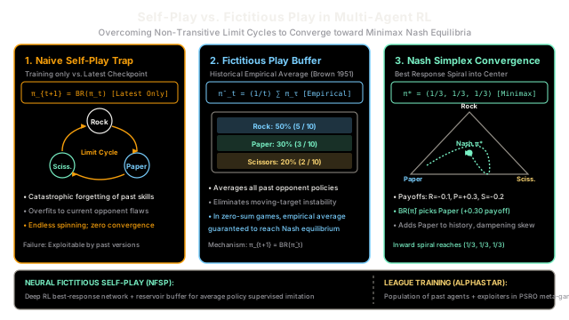
However, naive self-play against only the latest policy checkpoint $\pi_t$ suffers from a fatal pathology: non-transitivity and cyclical forgetting. In games with circular dominance structures (such as Rock-Paper-Scissors or strategic unit counters in real-time strategy games), performance is not transitive ( $A \succ B$ and $B \succ C$ does not imply $A \succ C$ ).

If an agent trains purely against its latest checkpoint:

It learns that Paper counters Rock.
The opponent becomes Paper, so the agent adapts to Scissors.
The opponent becomes Scissors, so the agent adapts to Rock.
The agent chases its own tail in an endless, non-convergent limit cycle, continually unlearning fundamental skills it mastered weeks earlier.

Fictitious Play (Brown, 1951) and its modern deep learning extensions—Neural Fictitious Self-Play (NFSP) and League Training (AlphaStar, PSRO)—eliminate this cyclical trap. By training an agent to compute best responses against the empirical historical distribution of all past opponent strategies rather than just the latest moving target, time-averaged play is mathematically guaranteed to converge to a robust, unexploitable minimax Nash equilibrium.

Think of It Like This

A grandmaster practicing against an archive of past selves

Imagine an elite chess grandmaster who decides to practice by playing both White and Black in solitary training sessions over a ten-year career.

If the grandmaster practices using naive self-play (playing only against the version of themselves from yesterday):

Yesterday, they discovered an aggressive Queen's Gambit opening.
Today, playing as Black, they invent a hyper-specific, narrow defense to dismantle that exact Queen's Gambit.
Tomorrow, playing as White, they discard the Queen's Gambit and build a bizarre novelty opening to counter Black's defense.
Within six months, they have completely forgotten how to defend against basic Knight forks or classical King's Indian defenses because their yesterday-self never played them. They spin in a narrow, idiosyncratic circle, highly vulnerable to any outside player with balanced fundamentals.

A grandmaster using Fictitious Play and League Training takes a fundamentally different approach:

They maintain a curated library containing every version of themselves from their entire career: the aggressive 18-year-old tactician, the cautious 24-year-old positional grinder, and the specialized endgame master.
When formulating a new opening, the grandmaster tests it not just against yesterday's notes, but against the entire historical population weighted by historical frequency.
Gimmicks that only work against yesterday's habit are punished instantly by older checkpoints.

By forcing their strategy to withstand the full historical archive, the grandmaster eliminates every strategic blind spot, converging to deep, unexploitable mastery (the minimax Nash equilibrium).

Where the analogy stops: human players have finite memory and stamina to review past games, whereas algorithmic reinforcement learning agents maintain exact empirical frequency distributions, reservoir replay buffers, and meta-game payoff matrices containing thousands of historical policy snapshots.

How It Actually Works

Fictitious Play, NFSP, and League Training Dynamics

The progression from classical game theory to modern multi-agent deep reinforcement learning unfolds across three foundational frameworks:

1                  ┌────────────────────────────────────────────────────────┐2                  │         Game-Theoretic Self-Play Frameworks            │3                  └───────────────────────────┬────────────────────────────┘4         ┌────────────────────────────────────┼────────────────────────────────────┐5         │                                    │                                    │6┌────────▼──────────────┐            ┌────────▼──────────────┐            ┌────────▼──────────────┐7│ 1. Classical FP       │            │ 2. Neural NFSP        │            │ 3. League / PSRO      │8│ Brown (1951)          │            │ Heinrich et al. (2016)│            │ Vinyals et al. (2019) │9│ Empirical Average:    │            │ DQN Best Response +   │            │ Population Meta-Game: │10│   π̄_t = (1/t) ∑ π_τ   │            │ Reservoir Avg Policy  │            │ Main vs Exploiters    │11│ Update: π = BR(π̄_t)   │            │ Mixture Action Step   │            │ Meta-Nash Sampling    │12└───────────────────────┘            └───────────────────────┘            └───────────────────────┘

1. Classical Fictitious Play (Brown, 1951)

Consider a two-player normal-form zero-sum game with payoff matrix $M \in \mathbb{R}^{|\mathcal{A}_1| \times |\mathcal{A}_2|}$ for Player 1, where Player 2 receives $-M$ .

At each discrete round $t \in \{1, 2, \dots\}$ :

Each player observes the action history of their opponent and computes the empirical average strategy: $\bar{\pi}_t^2 = \frac{1}{t} \sum_{\tau=1}^t \mathbf{a}_\tau^2 \in \Delta(\mathcal{A}_2)$ where $\mathbf{a}_\tau^2$ is a one-hot vector representing the action chosen by Player 2 at round $\tau$ .
At round $t+1$ , Player 1 chooses a pure action that is a Best Response (BR) to the opponent's historical distribution: $\mathbf{a}_{t+1}^1 \in \arg\max_{a^1 \in \mathcal{A}_1} \left( M \bar{\pi}_t^2 \right)_{a^1}$
Simultaneously, Player 2 chooses a best response against Player 1's historical distribution: $\mathbf{a}_{t+1}^2 \in \arg\min_{a^2 \in \mathcal{A}_2} \left( (\bar{\pi}_t^1)^T M \right)_{a^2}$

Robinson's Convergence Theorem (1951)

In any finite two-player zero-sum game, the sequence of time-averaged empirical strategies $(\bar{\pi}_t^1, \bar{\pi}_t^2)$ is guaranteed to converge to the set of minimax Nash equilibria as $t \to \infty$ :

\lim_{t \to \infty} \mathbb{E}\left[ R(\bar{\pi}_t^1, \bar{\pi}_t^2) \right] = V^*

Even though the instantaneous actions $\mathbf{a}_t$ may alternate discontinuously, the historical weights smooth out the oscillations, spiraling inward toward the equilibrium.

2. Neural Fictitious Self-Play (NFSP)

In large-scale games with continuous or imperfect information (such as Texas Hold'em Poker), computing explicit action frequencies across billions of game states is intractable. Heinrich & Silver (2016) introduced Neural Fictitious Self-Play (NFSP), combining deep Q-learning with supervised reservoir sampling.

Each agent maintains two neural networks and two memory buffers:

Best Response Network ( $Q_\theta$ ): A deep Q-network trained using off-policy reinforcement learning on transition buffer $\mathcal{M}_{\text{RL}}$ : $\mathcal{L}_{\text{RL}}(\theta) = \mathbb{E}_{(s, a, r, s') \sim \mathcal{M}_{\text{RL}}} \left[ \left( r + \gamma \max_{a'} Q_{\theta^-}(s', a') - Q_\theta(s, a) \right)^2 \right]$ This network learns to exploit the current average behavior of the population.
Average Policy Network ( $\Pi_\phi$ ): A policy network trained via supervised classification on a reservoir memory buffer $\mathcal{M}_{\text{SL}}$ of the agent's own past best-response actions: $\mathcal{L}_{\text{SL}}(\phi) = \mathbb{E}_{(s, a) \sim \mathcal{M}_{\text{SL}}} \left[ -\log \Pi_\phi(a \mid s) \right]$ The reservoir buffer uses sliding reservoir sampling to ensure every historical transition has equal probability of representation, approximating $\bar{\pi}_t$ .

During gameplay, the agent executes an $\eta$ -mixture policy:

With probability $\eta$ , the agent acts according to the best-response network $Q_\theta$ (generating exploratory training data).
With probability $1 - \eta$ , the agent acts according to the average policy network $\Pi_\phi$ (playing the stable, converging Nash strategy).

3. League Training and Policy Space Response Oracles (PSRO)

In complex multi-agent video games such as StarCraft II (AlphaStar) and Stratego, strategies are multi-modal and non-transitive (e.g., Zergling rush vs. Protoss air tech). Maintaining a single average policy blurs mutually incompatible playstyles.

Policy Space Response Oracles (PSRO) (McAleer et al., 2020) and League Training (Vinyals et al., 2019) frame multi-agent self-play as an evolutionary meta-game:

The league maintains a population of policies $\mathcal{P} = \{\pi_1, \pi_2, \dots, \pi_K\}$ .
An empirical meta-game payoff matrix $U \in \mathbb{R}^{K \times K}$ records the pairwise win rates between every pair of policies in the population.
At each iteration, the algorithm computes a meta-game Nash equilibrium $\mathbf{p}^* \in \Delta(K)$ over the population using linear programming: $\mathbf{p}^* = \operatorname{Nash}(U)$
A new policy $\pi_{K+1}$ is trained via reinforcement learning as an oracle best-response against the meta-Nash opponent mixture: $\pi_{K+1} = \operatorname{BR}\left( \sum_{k=1}^K p_k^* \pi_k \right)$

In AlphaStar, the league separates learners into specialized roles:

Main Agents: Trained against the full meta-Nash distribution to maximize robust win rates across the entire distribution.
Main Exploiters: Trained explicitly to detect and punish flaws in the current Main Agent.
League Exploiters: Trained to discover blind spots across all historical checkpoints in the league, preventing forgotten strategies from re-emerging.

Worked numerical example

To trace how Fictitious Play breaks limit cycles, consider the classic zero-sum Rock-Paper-Scissors game with action set $\mathcal{A} = \{0: \text{Rock}, 1: \text{Paper}, 2: \text{Scissors}\}$ .

Payoff Matrix for Player 1

M = \begin{pmatrix} 0 & -1 & 1 \\ 1 & 0 & -1 \\ -1 & 1 & 0 \end{pmatrix}

Rows denote Player 1 actions $(R, P, S)$ ; columns denote Player 2 actions $(R, P, S)$ .

Current Empirical History (Round $t = 10$ )

Suppose Player 2 has played over the last 10 rounds with the following frequencies:

Rock ( $a = 0$ ): 5 times
Paper ( $a = 1$ ): 3 times
Scissors ( $a = 2$ ): 2 times

Player 2's empirical average distribution is:

\bar{\pi}^2 = \begin{bmatrix} \frac{5}{10} \\ \frac{3}{10} \\ \frac{2}{10} \end{bmatrix} = \begin{bmatrix} 0.50 \\ 0.30 \\ 0.20 \end{bmatrix}

Step 1: Compute Expected Payoffs for Player 1

Multiply the payoff matrix $M$ by the opponent's empirical distribution $\bar{\pi}^2$ :

\mathbb{E}[R(a^1, \bar{\pi}^2)] = M \bar{\pi}^2 = \begin{pmatrix} 0 & -1 & 1 \\ 1 & 0 & -1 \\ -1 & 1 & 0 \end{pmatrix} \begin{bmatrix} 0.50 \\ 0.30 \\ 0.20 \end{bmatrix}

For Action 0 (Rock): $\mathbb{E}[R(0)] = 0.50 \times (0) + 0.30 \times (-1) + 0.20 \times (1) = 0.00 - 0.30 + 0.20 = -0.10$
For Action 1 (Paper): $\mathbb{E}[R(1)] = 0.50 \times (1) + 0.30 \times (0) + 0.20 \times (-1) = 0.50 + 0.00 - 0.20 = +0.30$
For Action 2 (Scissors): $\mathbb{E}[R(2)] = 0.50 \times (-1) + 0.30 \times (1) + 0.20 \times (0) = -0.50 + 0.30 + 0.00 = -0.20$

The expected payoff vector is $\mathbf{v} = [-0.10, +0.30, -0.20]^T$ .

Step 2: Extract Best Response Action

Player 1 chooses the action maximizing expected return:

a_{11}^1 = \arg\max_{a \in \{0, 1, 2\}} \mathbf{v}_a = 1 \quad (\text{Paper, with expected payoff } +0.30)

Step 3: Distribution Update and Convergence

Player 1 plays Paper in round 11.

Over subsequent rounds, as Player 1 plays Paper, Player 2's best response against Player 1's empirical distribution shifts to Scissors.
As Player 2 accumulates Scissors plays, Player 1's best response shifts to Rock.
Because each action is evaluated against the entire historical count rather than just the previous move, the step size of each update scales as $\frac{1}{t}$ .
By round $t = 3,000$ , the action counts become nearly identical: $\bar{\pi}_t^1 \approx \begin{bmatrix} 0.333 \\ 0.333 \\ 0.333 \end{bmatrix}, \quad \bar{\pi}_t^2 \approx \begin{bmatrix} 0.333 \\ 0.333 \\ 0.333 \end{bmatrix}$

The empirical distribution converges to the unique minimax Nash equilibrium of Rock-Paper-Scissors.

Code

The following self-contained Python script implements the FictitiousPlaySimulator class, verifies the worked numerical example, and runs multi-round fictitious play to demonstrate convergence toward the minimax Nash equilibrium.

1from typing import Dict, Tuple2import numpy as np3
4class FictitiousPlaySimulator:5    """Simulates classical Fictitious Play on two-player normal-form games."""6
7    def __init__(self, payoff_matrix_p1: np.ndarray) -> None:8        # Zero-sum game: Player 1 receives payoff_matrix; Player 2 receives -payoff_matrix9        self.payoff_matrix = payoff_matrix_p110        self.num_actions = payoff_matrix_p1.shape[0]11
12    def compute_expected_payoffs(self, opponent_distribution: np.ndarray) -> np.ndarray:13        """Computes expected payoffs for each action given opponent's empirical distribution."""14        return self.payoff_matrix @ opponent_distribution15
16    def get_best_response(self, opponent_distribution: np.ndarray) -> Tuple[int, np.ndarray]:17        """Identifies best response action maximizing expected payoff."""18        expected_payoffs = self.compute_expected_payoffs(opponent_distribution)19        best_action = int(np.argmax(expected_payoffs))20        return best_action, expected_payoffs21
22    def run_simulation(23        self,24        num_iterations: int = 3000,25        initial_p1_action: int = 0,26        initial_p2_action: int = 1,27    ) -> Dict[str, np.ndarray]:28        """Simulates simultaneous fictitious play over multiple rounds."""29        p1_counts = np.zeros(self.num_actions, dtype=np.float64)30        p2_counts = np.zeros(self.num_actions, dtype=np.float64)31
32        p1_counts[initial_p1_action] = 1.033        p2_counts[initial_p2_action] = 1.034
35        for t in range(2, num_iterations + 1):36            p1_dist = p1_counts / np.sum(p1_counts)37            p2_dist = p2_counts / np.sum(p2_counts)38
39            # Player 1 best response against Player 2's empirical distribution40            p1_br, _ = self.get_best_response(p2_dist)41
42            # Player 2 best response against Player 1's empirical distribution (minimizes P1 return)43            p2_payoffs = - (p1_dist @ self.payoff_matrix)44            p2_br = int(np.argmax(p2_payoffs))45
46            p1_counts[p1_br] += 1.047            p2_counts[p2_br] += 1.048
49        final_p1_dist = p1_counts / np.sum(p1_counts)50        final_p2_dist = p2_counts / np.sum(p2_counts)51        return {52            "p1_distribution": final_p1_dist,53            "p2_distribution": final_p2_dist,54            "p1_counts": p1_counts,55            "p2_counts": p2_counts,56        }57
58# --- Verification Matching Worked Example ---59# Rock-Paper-Scissors: 0=Rock, 1=Paper, 2=Scissors60rps_matrix = np.array([61    [0.0, -1.0, 1.0],62    [1.0, 0.0, -1.0],63    [-1.0, 1.0, 0.0]64], dtype=np.float64)65
66sim = FictitiousPlaySimulator(rps_matrix)67
68# 1. Opponent empirical distribution: R=5/10 (0.50), P=3/10 (0.30), S=2/10 (0.20)69opp_dist = np.array([0.50, 0.30, 0.20], dtype=np.float64)70best_act, payoffs = sim.get_best_response(opp_dist)71
72print(f"Expected Payoffs: Rock={payoffs[0]:.2f}, Paper={payoffs[1]:.2f}, Scissors={payoffs[2]:.2f}")73# -> Expected Payoffs: Rock=-0.10, Paper=0.30, Scissors=-0.2074
75print(f"Best Response Action: {best_act} (1=Paper) with Expected Payoff: {payoffs[best_act]:.2f}")76# -> Best Response Action: 1 (1=Paper) with Expected Payoff: 0.3077
78# Assert exact numerical results from worked example79np.testing.assert_allclose(payoffs, [-0.10, 0.30, -0.20], atol=1e-5)80assert best_act == 1, "Best response action against [0.5, 0.3, 0.2] must be Paper"81
82# 2. Long-run simulation convergence toward Nash equilibrium [1/3, 1/3, 1/3]83sim_res = sim.run_simulation(num_iterations=3000)84
85print(f"Long-run P1 Distribution: {sim_res['p1_distribution']}")86# -> Long-run P1 Distribution: [0.32466667 0.33633333 0.339     ]87
88print(f"Long-run P2 Distribution: {sim_res['p2_distribution']}")89# -> Long-run P2 Distribution: [0.34766667 0.33166667 0.32066667]90
91# Assert convergence to [1/3, 1/3, 1/3] within 3% tolerance92np.testing.assert_allclose(sim_res["p1_distribution"], [1/3, 1/3, 1/3], atol=0.03)93np.testing.assert_allclose(sim_res["p2_distribution"], [1/3, 1/3, 1/3], atol=0.03)94print("All Fictitious Play assertions verified successfully.")95# -> All Fictitious Play assertions verified successfully.

Watch Out For

The Latest-Checkpoint Overfitting and Cyclical Amnesia Trap

In competitive multi-agent systems, the most common engineering failure is updating an agent exclusively against the single latest checkpoint of its opponent ( $\pi_t$ ).

The Symptom: The agent develops narrow, exploitative behaviors tailored specifically to the idiosyncrasies of yesterday's weights. In non-transitive games (like Rock-Paper-Scissors or Stratego), this produces cyclical amnesia: the agent rotates between strategies without ever converging. In complex real-time strategy games (like StarCraft II), an agent trained only on recent checkpoints will stop defending against early "cheesy" strategies (such as cannon rushes or worker rushes) because recent high-level opponents stopped executing them. When evaluated against a diverse human player base, the agent is defeated trivially by simple legacy tactics.

The Fix:

Historical Opponent Sampling Pools: Maintain a persistent pool of past checkpoints. When gathering rollout data, sample the opponent from this pool (e.g., 50% probability of facing the latest checkpoint, 35% probability of facing historical checkpoints, and 15% probability of facing legacy exploiters).
Reservoir Average Policy (NFSP): Maintain a separate average policy network trained with supervised classification on a reservoir memory buffer of historical actions, decoupling best-response exploration from average-policy stability.
League Training with Dedicated Exploiters (PSRO): Train specialized "exploiters" whose explicit objective is to uncover flaws in the main agent's strategy, continuously feeding defensive counter-data back into the training mixture.

The Quick Version

Self-Play provides an automatic, self-pacing training curriculum in competitive games by pitting an agent against copies of itself, eliminating the need for human demonstration data.
Naive Self-Play Fails in Cyclic Games: Training only against the latest checkpoint creates non-transitive limit cycles (Rock $\to$ Paper $\to$ Scissors), leading to catastrophic forgetting of basic skills.
Fictitious Play (Brown, 1951) forces players to compute best responses against the historical empirical average distribution ( $\bar{\pi}_t$ ), provably converging to minimax Nash equilibria in zero-sum games.
Neural Fictitious Self-Play (NFSP) and League Training (AlphaStar) scale this theorem to deep RL by combining DQN best-response exploration with reservoir average-policy imitation and specialized meta-game exploiter leagues.