Trajectory Sampling

Rather than wasting computational budget updating every state in an enormous state space equally, trajectory sampling simulates rollouts using an internal environment model. This restricts planning updates exclusively to states that the agent will actually encounter under its current policy.

Why Does This Exist?

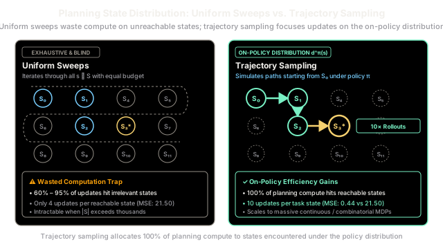
In model-based reinforcement learning and Dynamic Programming, planning algorithms improve value functions and policies by simulating transitions through an internal environment model. The traditional approach is uniform sweeping: the planner iterates through the entire state space $\mathcal{S}$ in an exhaustive round-robin fashion, applying Bellman backups to each state with equal frequency.

While uniform sweeping guarantees global convergence in small, toy Markov Decision Processes, it fails completely when scaled to practical problems:

The Curse of Irrelevant States: In realistic tasks, the state space $|\mathcal{S}|$ is combinatorial or massive. Worse, the vast majority of these states are either physically unreachable from starting conditions or represent bizarre, pathological configurations that an agent following a reasonable policy will never encounter.
Diluted Computational Budget: If an environment contains $1,000,000$ states but the agent only ever visits $1,000$ of them along plausible goal-oriented trajectories, uniform sweeping expends $99.9\%$ of its planning computation updating values for states that have literally zero impact on decision-making. Important bottleneck states receive only a trickle of updates.

Trajectory sampling exists to align the distribution of planning computation with the distribution of actual agent experience.

Instead of sweeping the state space uniformly, the agent uses its learned model to simulate complete episodes starting from initial states and selecting actions according to its current policy $\pi$ . By executing planning updates exclusively along these simulated rollouts, updates are distributed according to the on-policy state distribution $d^\pi(s)$ . States that are frequently visited under the policy receive intense, focused refinement, while unreachable states consume zero computational cycles.

Think of It Like This

The Continental GPS Router

Imagine programming a GPS navigation engine to compute the fastest driving route from Seattle to San Francisco.

A uniform sweeping router would load every intersection, dirt road, alleyway, and rural roundabout across the entire North American continent—from Anchorage, Alaska to Key West, Florida—into memory. It would iterate through every single crossroads in round-robin order, recalculating speed limits and traffic lights for all of them equally.

For hours, your computer fan would spin at maximum speed while the system calculated optimal left turns in southern Ohio and downtown Miami—intersections that have literally zero relevance to driving down the Pacific coast.

A trajectory sampling router operates with common sense:

It begins at your current Seattle coordinates ( $S_0$ ).
It projects prospective travel corridors southward along major highways (Interstate 5 and US-101), querying its road network model to simulate intersections along plausible paths toward San Francisco.
It refines junction choices along that prospective corridor, ignoring the millions of irrelevant roads in other states.

Because 100% of the processor's budget is concentrated on the corridor of reachable travel, you receive a near-optimal driving itinerary in milliseconds.

Where the analogy stops: Road networks have static, fixed highway layouts. In reinforcement learning, the environment's transition probabilities and rewards can be stochastic, and updating the policy alters which future states become reachable. Consequently, trajectory sampling must maintain sufficient exploratory action selection to prevent missing newly promising corridors.

How It Actually Works

The On-Policy Distribution and Simulated Rollout Mechanism

In planning frameworks such as Dyna-Q and Real-Time Dynamic Programming (RTDP), trajectory sampling generates simulated trajectories using the agent's learned or given model $\mathcal{M} = \langle p(s', r \mid s, a) \rangle$ .

The On-Policy State Distribution

Let an agent start at state $S_0 \sim \rho_0$ and follow target policy $\pi$ . The discounted on-policy state distribution $d^\pi(s)$ is defined as:

d^\pi(s) \doteq (1 - \gamma) \sum_{t=0}^\infty \gamma^t P(S_t = s \mid S_0 \sim \rho_0, \pi)

where:

$\rho_0$ is the starting state distribution.
$\gamma \in [0, 1)$ is the discount factor.
$P(S_t = s \mid S_0, \pi)$ is the probability that state $s$ is occupied at time step $t$ under policy $\pi$ .

When a planner samples trajectories according to $d^\pi(s)$ , the frequency of planning updates applied to state $s$ is directly proportional to its probability of being visited during actual task execution.

Algorithmic Flow of Trajectory Sampling Planning

At each planning cycle:

Initialize State: Sample a start state $S \sim \rho_0$ (or select the agent's current real-world state).
Rollout Loop: Until a terminal state is reached or horizon limit is met: a. Action Selection: Select action $A$ according to behavior policy $b(\cdot \mid S)$ (e.g., $\epsilon$ -greedy with respect to current $Q$ ): $A \sim b(\cdot \mid S)$ b. Model Query: Query the internal transition model to generate a simulated next state $S'$ and reward $R$ : $S', R \sim p(\cdot, \cdot \mid S, A)$ c. In-Place Planning Update: Update the action-value estimate $Q(S, A)$ using a sample backup: $Q(S, A) \leftarrow Q(S, A) + \alpha \left[ R + \gamma \max_{a'} Q(S', a') - Q(S, A) \right]$ (or alternatively apply a full expected Bellman backup if branching is small). d. Advance Simulation: Step forward along the simulated trajectory: $S \leftarrow S'$

The Short-Term vs. Long-Term Convergence Trade-off

Richard Sutton and Andrew Barto analyzed the fundamental trade-off between uniform sweeping and on-policy trajectory sampling (Section 8.6):

1Policy Value / Convergence2    ▲3    │                                  Trajectory Sampling (Fast early gains)4    │                         .────────────────────────────────────────────►5    │                   . - '6    │             . - '7    │       . - '                      Uniform Sweeps (Sluggish start, slow global convergence)8    │   . '                   .────────────────────────────────────────────►9    │  '          . - - - - '10    │ . - - - - '11    └──────────────────────────────────────────────────────────────► Planning Updates12      0               Low Budget (Practical)                  Infinite Budget (Asymptotic)

Under Low-to-Moderate Budgets: Trajectory sampling converges dramatically faster. By directing 100% of backups to reachable states along the current trajectory, the agent rapidly discovers a working policy to reach the goal.
Under Infinite Budgets: Uniform sweeping eventually guarantees that all states in $\mathcal{S}$ —even bizarre, unreachable corners—converge to their true Bellman values. However, because an optimal agent will never visit unreachable states anyway, investing compute to evaluate them provides zero performance benefit in real tasks.

Worked numerical comparison

Consider an environment with $10$ total discrete states: $\mathcal{S} = \{S_0, S_1, \dots, S_9\}$ .

The task begins at start state $S_0$ .
Under policy $\pi$ , the reachable chain is: $S_0 \xrightarrow{} S_1 \xrightarrow{} S_2 \xrightarrow{} S_3 \xrightarrow{} \text{Terminal}$ .
States $S_4, S_5, \dots, S_9$ ( $6$ states, $60\%$ of the state space) are unreachable or irrelevant loops with zero reward.
Transition dynamics: Reward is $0.0$ on intermediate transitions, with a terminal reward of $+10.0$ upon exiting $S_3$ .
Discount factor: $\gamma = 0.9$ . Step-size learning rate: $\alpha = 0.5$ .

True Optimal Values on Reachable States

Working backward from the goal:

$V^*(S_3) = 10.0000$
$V^*(S_2) = 0.9 \times 10.0000 = \mathbf{9.0000}$
$V^*(S_1) = 0.9 \times 9.0000 = \mathbf{8.1000}$
$V^*(S_0) = 0.9 \times 8.1000 = \mathbf{7.2900}$

All states are initialized to $0.0000$ . The planner is allocated a budget of exactly $40$ planning updates.

Case A: Uniform Sweeping ( $40$ Updates)

With $10$ total states, a uniform round-robin sweep updates each state in sequence ( $S_0, S_1, \dots, S_9$ ) across $4$ complete passes ( $40 / 10 = 4$ updates per state).

Reachable states ( $S_0 \dots S_3$ ): Each state receives only $4$ updates.
Unreachable states ( $S_4 \dots S_9$ ): Absorb $24$ updates ( $60\%$ of total budget) calculating transitions for states the agent never visits!

After $4$ passes, the value estimates on the reachable chain are:

$V(S_3) = 9.3750$
$V(S_2) = 6.1875$
$V(S_1) = 2.5312$
$V(S_0) = 0.4556$

Mean Squared Error (MSE) on the task states:

\text{MSE}_{\text{uniform}} = \frac{1}{4} \left[ (0.4556 - 7.29)^2 + (2.5312 - 8.1)^2 + (6.1875 - 9.0)^2 + (9.3750 - 10.0)^2 \right] = \mathbf{21.5051}

The start state $S_0$ has barely registered that a goal exists ( $0.4556$ vs true $7.2900$ ) because updates were diluted across the entire state space.

Case B: Trajectory Sampling ( $40$ Updates)

The planner simulates trajectories starting from $S_0$ following policy $\pi$ :

S_0 \to S_1 \to S_2 \to S_3 \to \text{Terminal}

Each simulated rollout executes $4$ state updates. Within the $40$ -update budget, the planner completes $10$ full trajectories ( $40 / 4 = 10$ ).

Reachable states ( $S_0 \dots S_3$ ): Each state receives $10$ focused updates ( $2.5\times$ more than uniform sweeping).
Unreachable states ( $S_4 \dots S_9$ ): Absorb $0$ updates ( $0\%$ wasted compute).

After $10$ simulated rollouts, the value estimates are:

$V(S_3) = 9.9902$
$V(S_2) = 8.9033$
$V(S_1) = 7.6570$
$V(S_0) = 6.0370$

Mean Squared Error (MSE) on the task states:

\text{MSE}_{\text{trajectory}} = \frac{1}{4} \left[ (6.0370 - 7.29)^2 + (7.6570 - 8.1)^2 + (8.9033 - 9.0)^2 + (9.9902 - 10.0)^2 \right] = \mathbf{0.4439}

Conclusion: For the exact same computational budget ( $40$ updates), trajectory sampling achieves a $48\times$ reduction in prediction error ( $\text{MSE } 0.4439$ vs $21.5051$ ) and brings the start state value close to convergence.

Code

1from typing import Dict, List, Tuple2
3
4def evaluate_planning_convergence(5    num_total_states: int,6    reachable_chain: List[int],7    gamma: float = 0.9,8    alpha: float = 0.5,9    terminal_reward: float = 10.0,10    total_budget: int = 40,11) -> Tuple[Dict[str, float], Dict[str, float]]:12    """Compare Uniform Sweeping vs Trajectory Sampling on a fixed computational budget.13
14    Args:15        num_total_states: Total size of discrete state space |S|.16        reachable_chain: Sequential state ids forming the task trajectory.17        gamma: Discount factor in [0, 1].18        alpha: Planning update step-size.19        terminal_reward: Reward achieved upon reaching terminal state.20        total_budget: Fixed number of planning backups allowed.21
22    Returns:23        Tuple of (uniform_results_summary, trajectory_results_summary).24    """25    chain_len = len(reachable_chain)26
27    # 1. Uniform Sweeps (Exhaustive round-robin across all states)28    v_uniform: Dict[int, float] = {s: 0.0 for s in range(num_total_states)}29    rounds = total_budget // num_total_states30    for _ in range(rounds):31        for s in range(num_total_states):32            if s in reachable_chain:33                idx = reachable_chain.index(s)34                if idx == chain_len - 1:35                    target = terminal_reward36                else:37                    next_s = reachable_chain[idx + 1]38                    target = gamma * v_uniform[next_s]39            else:40                target = gamma * v_uniform[s]  # Irrelevant self-looping state41            v_uniform[s] += alpha * (target - v_uniform[s])42
43    # 2. Trajectory Sampling (Simulated on-policy rollouts starting from S0)44    v_traj: Dict[int, float] = {s: 0.0 for s in range(num_total_states)}45    trajectories = total_budget // chain_len46    for _ in range(trajectories):47        for idx, s in enumerate(reachable_chain):48            if idx == chain_len - 1:49                target = terminal_reward50            else:51                next_s = reachable_chain[idx + 1]52                target = gamma * v_traj[next_s]53            v_traj[s] += alpha * (target - v_traj[s])54
55    # Compute Ground Truth V* on reachable chain56    true_v: Dict[int, float] = {}57    curr_val = terminal_reward58    for s in reversed(reachable_chain):59        true_v[s] = curr_val60        curr_val *= gamma61
62    mse_uniform = sum((v_uniform[s] - true_v[s]) ** 2 for s in reachable_chain) / chain_len63    mse_traj = sum((v_traj[s] - true_v[s]) ** 2 for s in reachable_chain) / chain_len64
65    res_uniform = {66        "mse": round(mse_uniform, 4),67        "v_start": round(v_uniform[reachable_chain[0]], 4),68        "wasted_updates": total_budget - (rounds * chain_len),69    }70    res_traj = {71        "mse": round(mse_traj, 4),72        "v_start": round(v_traj[reachable_chain[0]], 4),73        "wasted_updates": 0,74    }75    return res_uniform, res_traj76
77
78# Execute simulation matching the worked numerical comparison79u_res, t_res = evaluate_planning_convergence(80    num_total_states=10,81    reachable_chain=[0, 1, 2, 3],82    gamma=0.9,83    alpha=0.5,84    terminal_reward=10.0,85    total_budget=40,86)87
88# Automated verification89assert u_res["wasted_updates"] == 2490assert t_res["wasted_updates"] == 091assert abs(u_res["v_start"] - 0.4556) < 1e-492assert abs(t_res["v_start"] - 6.0370) < 1e-493assert abs(u_res["mse"] - 21.5051) < 1e-494assert abs(t_res["mse"] - 0.4439) < 1e-495
96print(f"Uniform Sweeps    | Start V(S0): {u_res['v_start']:6.4f} | MSE: {u_res['mse']:7.4f} | Wasted Updates: {u_res['wasted_updates']}")97print(f"Trajectory Sample | Start V(S0): {t_res['v_start']:6.4f} | MSE: {t_res['mse']:7.4f} | Wasted Updates: {t_res['wasted_updates']}")98
99# -> Uniform Sweeps    | Start V(S0): 0.4556 | MSE: 21.5051 | Wasted Updates: 24100# -> Trajectory Sample | Start V(S0): 6.0370 | MSE:  0.4439 | Wasted Updates: 0

Watch Out For

The Trajectory Sampling Myopia and Exploration Trap

While trajectory sampling dramatically outperforms uniform sweeping by focusing on on-policy states, purely greedy trajectory sampling ( $\epsilon = 0$ ) creates a severe failure mode: policy lock-in.

The Failure Mode: If the behavior policy during simulated rollouts is purely greedy with respect to initial, inaccurate value estimates, the planner repeatedly simulates the exact same suboptimal trajectory.

Because states off this chosen path are never visited in simulation, their values are never updated. Even if a neighboring branch contains a massive positive reward, the planner remains completely blind to it. The agent becomes trapped in a self-fulfilling prophecy: it only plans along paths it believes are good, and it only updates paths it plans along.

Concrete Fix:

Always use an exploratory rollout policy: During model simulation, select actions using $\epsilon$ -greedy exploration ( $\epsilon \in [0.1, 0.2]$ ) or Boltzmann softmax exploration. This guarantees that simulated trajectories occasionally branch into unvisited states, allowing the model to discover shortcut paths.
Combine with Prioritized Sweeping: In deterministic or tabular domains, pair trajectory sampling with a priority queue (such as Prioritized Sweeping) that tracks states with large Bellman error $\delta$ . If an exploratory rollout uncovers a large reward, the priority queue immediately propagates that error backward across all predecessor states, preventing lock-in.

The Quick Version

Uniform sweeps waste over $90\%$ of planning computation in large state spaces by updating unreachable or irrelevant states.
Trajectory sampling simulates rollouts using an internal environment model, distributing updates according to the on-policy state distribution $d^\pi(s)$ .
States along realistic task trajectories receive dense, concentrated planning updates, achieving near-optimal policies in orders of magnitude fewer operations.
Rollout action selection must remain exploratory ( $\epsilon$ -greedy) to avoid myopic lock-in on early suboptimal trajectories.