Off-Policy Importance Sampling

Evaluate a target policy without ever running it by observing a different behavior policy and re-weighting returns by action probability ratios.

Why Does This Exist?

In reinforcement learning, learning on-policy creates a persistent conflict between exploration and control. To find an optimal policy, an agent must take exploratory, potentially suboptimal actions. But to evaluate or execute an optimal policy, the agent must act greedily.

In on-policy methods, an agent evaluates the very policy that dictates its behavior. If that behavior explores, the agent evaluates an exploratory policy rather than the true optimal policy. Furthermore, all historical data collected under previous policies becomes obsolete and must be discarded whenever the agent updates its policy.

Off-policy prediction resolves this dilemma by decoupling the learning process into two distinct roles:

Target Policy ( $\pi$ ): The policy being evaluated, optimized, or learned (often a deterministic, greedy, or candidate control policy).
Behavior Policy ( $b$ ): The policy used to generate actions and gather experience in the environment (often exploratory, safe, or an existing legacy controller).

Because the agent follows behavior policy $b$ , the raw observed returns reflect the distribution induced by $b$ , not $\pi$ . Without correction, averaging these returns yields a heavily biased estimate of $\pi$ 's value. Importance sampling provides the exact statistical re-weighting needed to transform sample returns gathered under $b$ into an unbiased estimate of the value under $\pi$ .

Think of It Like This

Demographic Polling Adjustments

Imagine a polling organization wants to predict how the entire voting electorate (the target policy $\pi$ ) will vote on upcoming referendums. Due to collection constraints, their field survey only managed to interview college students on campus (the behavior policy $b$ ).

In the surveyed student sample, 80% support public transit expansion and 20% support highway expansions. However, historical census data reveals that in the general electorate, only 40% prioritize public transit while 60% prioritize highway expansions.

If the pollsters simply averaged the raw student responses, their forecast for the general election would be hopelessly skewed. To correct for this sampling bias, they apply an adjustment factor to each response:

A vote for public transit is multiplied by $\frac{0.40}{0.80} = 0.50$ (down-weighted because transit supporters were overrepresented).
A vote for highway expansion is multiplied by $\frac{0.60}{0.20} = 3.00$ (up-weighted because highway supporters were underrepresented).

By multiplying every recorded response by the ratio $\frac{\pi(\text{group})}{b(\text{group})}$ , the pollsters compute an unbiased estimate of the general population's preferences using data from a completely different group.

Where the analogy stops: Demographic polling evaluates a single, independent choice per respondent. In reinforcement learning, an episode is a sequential chain of decisions over time. The agent must multiply these probability ratios across every successive time step of the trajectory, creating a compounding product that can rapidly fluctuate.

How It Actually Works

Target Policy vs. Behavior Policy and the Importance Sampling Ratio

Let $\pi(a \mid s)$ denote the probability of choosing action $a$ in state $s$ under the target policy, and let $b(a \mid s)$ denote the corresponding probability under the behavior policy.

To estimate the value function $V^\pi(s)$ from episodes generated by $b$ , we must satisfy the coverage assumption: $\pi(a \mid s) > 0 \implies b(a \mid s) > 0 \quad \forall s \in \mathcal{S}, a \in \mathcal{A}(s)$

If the target policy $\pi$ could take an action in a state that the behavior policy $b$ never attempts ( $b(a \mid s) = 0$ ), the agent will never observe data for that transition, making it impossible to evaluate $\pi$ .

Consider an episode trajectory segment starting at time step $t$ and terminating at time $T$ : $\tau = (A_t, S_{t+1}, A_{t+1}, \dots, S_T)$

Under behavior policy $b$ , the probability of observing this sequence of actions and states given starting state $S_t$ is: $\mathbb{P}(\tau \mid S_t, b) = \prod_{k=t}^{T-1} b(A_k \mid S_k) p(S_{k+1} \mid S_k, A_k)$ where $p(S_{k+1} \mid S_k, A_k)$ represents the environment's transition dynamics.

Under target policy $\pi$ , the probability of that identical trajectory would be: $\mathbb{P}(\tau \mid S_t, \pi) = \prod_{k=t}^{T-1} \pi(A_k \mid S_k) p(S_{k+1} \mid S_k, A_k)$

The importance sampling ratio $\rho_{t:T-1}$ is defined as the relative probability of the trajectory under $\pi$ compared to $b$ : $\rho_{t:T-1} = \frac{\prod_{k=t}^{T-1} \pi(A_k \mid S_k) p(S_{k+1} \mid S_k, A_k)}{\prod_{k=t}^{T-1} b(A_k \mid S_k) p(S_{k+1} \mid S_k, A_k)} = \prod_{k=t}^{T-1} \frac{\pi(A_k \mid S_k)}{b(A_k \mid S_k)}$

The transition probabilities $p(S_{k+1} \mid S_k, A_k)$ are identical in numerator and denominator and cancel out completely. This makes importance sampling fully model-free: we do not need to know the environment's transition probabilities.

The expected value of the return $G_t$ under behavior policy $b$ , scaled by $\rho_{t:T-1}$ , matches the true expectation under target policy $\pi$ : $\mathbb{E}_b[\rho_{t:T-1} G_t \mid S_t = s] = \sum_{\tau} \mathbb{P}(\tau \mid s, b) \left( \frac{\mathbb{P}(\tau \mid s, \pi)}{\mathbb{P}(\tau \mid s, b)} G_t(\tau) \right) = \sum_{\tau} \mathbb{P}(\tau \mid s, \pi) G_t(\tau) = V^\pi(s)$

In ordinary importance sampling, an agent samples $N$ episodes starting from state $s$ under behavior policy $b$ and computes the empirical mean: $V(s) = \frac{1}{N} \sum_{i=1}^N \rho_{t(i):T(i)-1}^{(i)} G_t^{(i)}$

Worked numerical example

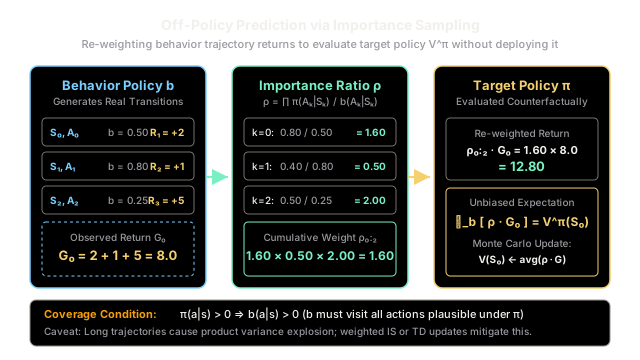
Consider a 3-step episode generated under behavior policy $b$ with discount factor $\gamma = 1.0$ : $\tau = (S_0, A_0, R_1=2, S_1, A_1, R_2=1, S_2, A_2, R_3=5, S_3)$

The observed unweighted return from $S_0$ is: $G_0 = R_1 + R_2 + R_3 = 2.0 + 1.0 + 5.0 = 8.0$

The target policy $\pi$ and behavior policy $b$ assign the following probabilities to the actions chosen at each time step:

Step $k = 0$ at state $S_0$ taking action $A_0$ : $\pi(A_0 \mid S_0) = 0.80, \quad b(A_0 \mid S_0) = 0.50 \implies \frac{\pi(A_0 \mid S_0)}{b(A_0 \mid S_0)} = \frac{0.80}{0.50} = 1.60$
Step $k = 1$ at state $S_1$ taking action $A_1$ : $\pi(A_1 \mid S_1) = 0.40, \quad b(A_1 \mid S_1) = 0.80 \implies \frac{\pi(A_1 \mid S_1)}{b(A_1 \mid S_1)} = \frac{0.40}{0.80} = 0.50$
Step $k = 2$ at state $S_2$ taking action $A_2$ : $\pi(A_2 \mid S_2) = 0.50, \quad b(A_2 \mid S_2) = 0.25 \implies \frac{\pi(A_2 \mid S_2)}{b(A_2 \mid S_2)} = \frac{0.50}{0.25} = 2.00$

The cumulative trajectory importance sampling ratio is the product across all three steps: $\rho_{0:2} = 1.60 \times 0.50 \times 2.00 = 1.60$

The re-weighted return contribution from this trajectory is: $\rho_{0:2} G_0 = 1.60 \times 8.0 = 12.80$

Now suppose a second episode starting from $S_0$ yields raw return $G_0^{(2)} = 4.0$ with cumulative ratio $\rho_{0:T-1}^{(2)} = 0.75$ , giving a re-weighted return of $0.75 \times 4.0 = 3.00$ .

The ordinary importance sampling estimate of $V^\pi(S_0)$ across these two episodes is: $V(S_0) = \frac{12.80 + 3.00}{2} = 7.90$

Even though the target policy $\pi$ was never executed in the environment, the scaled returns provide an unbiased estimate of how well $\pi$ performs.

Code

1from typing import List, NamedTuple2
3class Transition(NamedTuple):4    state: str5    action: str6    reward: float7    pi_prob: float  # Target policy probability: pi(a|s)8    b_prob: float   # Behavior policy probability: b(a|s)9
10def evaluate_trajectory_importance_sampling(11    trajectory: List[Transition], 12    gamma: float = 1.013) -> tuple[float, float, float]:14    """15    Computes raw return G_0, cumulative importance sampling ratio rho,16    and the re-weighted return rho * G_0 for off-policy prediction.17    """18    rho = 1.019    for step in trajectory:20        assert step.b_prob > 0.0, "Coverage violation: b(a|s) must be > 0"21        ratio = step.pi_prob / step.b_prob22        rho *= ratio23
24    # Calculate discounted return G_025    g = 0.026    for t, step in enumerate(trajectory):27        g += (gamma ** t) * step.reward28
29    weighted_return = rho * g30    return g, rho, weighted_return31
32def ordinary_importance_sampling_estimate(33    episodes: List[List[Transition]], 34    gamma: float = 1.035) -> float:36    """Computes the sample average of weighted returns across episodes."""37    total_weighted = sum(38        evaluate_trajectory_importance_sampling(ep, gamma)[2] 39        for ep in episodes40    )41    return total_weighted / len(episodes)42
43# Episode 1 (from worked example)44ep1 = [45    Transition(state="S0", action="A0", reward=2.0, pi_prob=0.80, b_prob=0.50),46    Transition(state="S1", action="A1", reward=1.0, pi_prob=0.40, b_prob=0.80),47    Transition(state="S2", action="A2", reward=5.0, pi_prob=0.50, b_prob=0.25),48]49
50# Episode 251ep2 = [52    Transition(state="S0", action="A1", reward=1.0, pi_prob=0.30, b_prob=0.40),53    Transition(state="S1", action="A0", reward=3.0, pi_prob=1.00, b_prob=1.00),54]55
56g1, rho1, weighted1 = evaluate_trajectory_importance_sampling(ep1)57g2, rho2, weighted2 = evaluate_trajectory_importance_sampling(ep2)58
59print(f"Episode 1: Raw Return = {g1:.2f}, rho = {rho1:.2f}, Weighted = {weighted1:.2f}")60print(f"Episode 2: Raw Return = {g2:.2f}, rho = {rho2:.2f}, Weighted = {weighted2:.2f}")61
62v_estimate = ordinary_importance_sampling_estimate([ep1, ep2])63print(f"Estimated V^pi(S0) = {v_estimate:.2f}")64
65# -> Expected output:66# Episode 1: Raw Return = 8.00, rho = 1.60, Weighted = 12.8067# Episode 2: Raw Return = 4.00, rho = 0.75, Weighted = 3.0068# Estimated V^pi(S0) = 7.90

Watch Out For

Exponential Variance Explosion Along Long Trajectories

Ordinary importance sampling is strictly unbiased, but its variance can be astronomically high or even theoretically infinite. Because the trajectory weight $\rho_{t:T-1} = \prod_{k=t}^{T-1} \frac{\pi(A_k \mid S_k)}{b(A_k \mid S_k)}$ is a product of ratios, small differences between $\pi$ and $b$ compound exponentially with trajectory length $T$ .

In long horizons, most trajectories under $b$ take at least one action that $\pi$ considers unlikely, causing $\rho$ to drop to $0$ . Conversely, an occasional trajectory aligns with high-probability actions under $\pi$ , producing an enormous $\rho$ value. The resulting empirical average oscillates wildly, requiring impractical numbers of samples to converge.

The Fix:

Switch to Weighted Importance Sampling (WIS), which divides by the sum of importance ratios ( $\sum_i \rho^{(i)}$ ) rather than the episode count $N$ . WIS introduces a mild bias but guarantees bounded weights and dramatically lower variance.
Use discounting-aware importance sampling or temporal-difference (TD) methods (such as Q-learning or Expected SARSA), which bootstrap after 1 step to avoid cumulative multi-step product expansion.

The Quick Version

Off-policy prediction evaluates a target policy $\pi$ using trajectory data generated by a separate behavior policy $b$ .
The coverage assumption requires $b(a \mid s) > 0$ for every state-action pair where $\pi(a \mid s) > 0$ .
The importance sampling ratio $\rho_{t:T-1} = \prod_{k=t}^{T-1} \frac{\pi(A_k \mid S_k)}{b(A_k \mid S_k)}$ cancels environment transition dynamics, enabling model-free re-weighting.
Ordinary importance sampling is strictly unbiased ( $\mathbb{E}_b[\rho G_t] = V^\pi(S_t)$ ), but suffers from extreme variance over long horizons due to compounding products of ratios.