Importance Sampling: Ordinary vs Weighted
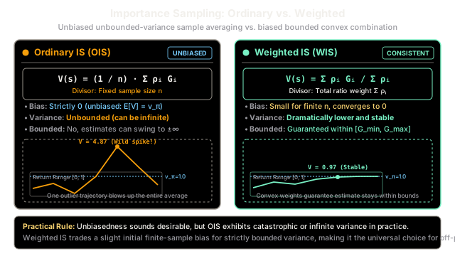
Ordinary importance sampling scales returns by raw probability ratios and divides by trajectory count, creating massive variance, whereas weighted importance sampling normalizes by the sum of ratios, trading initial bias for stable, bounded estimates.
Why Does This Exist?
Off-policy evaluation enables a reinforcement learning agent to estimate the value of a target policy using trajectory rollouts collected under a distinct, exploratory behavior policy . Because state-action paths are sampled according to rather than , their observed returns cannot simply be averaged together without adjustment; doing so would estimate rather than .
To correct for this distributional mismatch, importance sampling reweights each trajectory's return by the likelihood ratio of the action sequence under versus :
The mathematical dilemma arises in how to aggregate these reweighted returns:
- Ordinary Importance Sampling (OIS) takes the simple arithmetic average of the weighted returns across episodes, dividing by . While OIS is strictly unbiased (), its variance grows exponentially with the episode horizon . In multi-step tasks, the variance of can be unbounded or even infinite. A single rare trajectory with a massive ratio can inflate the sample mean by thousands of units, destroying estimation accuracy.
- Weighted Importance Sampling (WIS) divides the sum of weighted returns by the sum of importance ratios rather than the raw episode count . While WIS is biased for small sample sizes, this normalization converts the estimate into a convex combination of returns, guaranteeing that the estimate stays strictly bounded within the physical range of observed returns and slashing variance by orders of magnitude.
Understanding this bias-variance tradeoff is critical: in off-policy Monte Carlo learning, chasing zero bias with Ordinary IS frequently leads to non-converging algorithms, making Weighted IS the de facto standard in practice.
Think of It Like This
Estimating crowd height with raw multipliers versus a normalized weighted average
Imagine you want to calculate the average height of attendees at an international basketball tournament. However, you only have survey data collected outside a nearby coffee shop where most visitors were casual spectators, while only a few were 7-foot tall players.
Under the logic of Ordinary Importance Sampling, you calculate a representation multiplier for each demographic to correct for how underrepresented they were outside the coffee shop, multiply their height by this multiplier, and then divide the final sum by the raw headcount of people surveyed (). If you happen to interview just one 7-foot player whose demographic multiplier is , their single contribution adds feet to your running total! Dividing that total by your small survey size of people yields an estimated average crowd height of over feet. Because the denominator is a fixed headcount independent of the multipliers, a single outlier demographic blows the estimate completely outside the laws of human biology.
Under Weighted Importance Sampling, you divide the sum of weighted heights by the sum of all demographic multipliers. The multipliers now act as relative percentage shares rather than unconstrained expansion factors. Even if that 7-foot player carries a massive weight of , that exact same appears in the denominator alongside the other weights. The calculation remains a true weighted average, mathematically guaranteed to fall between the shortest person (say, 5'2") and tallest person (7'1") in your sample.
Where the analogy stops: In static human surveys, demographic weights are often pre-calculated constants. In reinforcement learning, the importance weight is a cumulative product of stochastic probabilities along an entire trajectory, meaning trajectory weights can easily span ten orders of magnitude within the exact same training run.
How It Actually Works
The Mathematical Formulation and Variance Divergence
Consider estimating the state-value function of a target policy from independent episodes generated by behavior policy , satisfying the coverage assumption: .
For each episode visiting state at time step , let represent the subsequent return, and let denote the full trajectory importance sampling ratio:
1. Ordinary Importance Sampling (OIS)
Ordinary importance sampling averages the reweighted returns directly across the trajectories:
Expectation (Unbiased)
Using the tower property and change of measure:
The bias of Ordinary Importance Sampling is strictly zero for any sample size .
Variance (Potentially Infinite)
The variance is:
Because is a product of per-step ratios , the second moment grows exponentially with trajectory length . If there exists any transition where , the variance of diverges to infinity as . When variance is infinite, sample averages do not converge reliably under the Central Limit Theorem.
2. Weighted Importance Sampling (WIS)
Weighted importance sampling normalizes by the empirical sum of importance sampling ratios:
(If , is defined to be ).
Bias (Non-Zero for Finite )
When and :
Taking the expectation with respect to the sampling policy :
With a single sample, the expectation of WIS equals the value of the behavior policy, not the target policy! Thus, WIS is biased for finite sample sizes.
Consistency (Asymptotic Convergence)
By the Strong Law of Large Numbers, as the sample count :
Therefore, the ratio of the empirical sums converges almost surely to the true value:
WIS is statistically consistent: its bias asymptotically vanishes to zero as more trajectories accumulate.
Bounded Range and Variance Reduction
Let . Since and , is a strict convex combination. Consequently:
The estimate is strictly bounded within the physical range of observed returns. Even if an extreme trajectory produces , its normalized weight , pulling the estimate toward rather than blowing up to infinity.
Worked numerical example
Let an agent evaluate state under target policy using off-policy trajectories collected by behavior policy . Suppose true target policy value is , and rewards are bounded such that all observed returns .
We observe 3 trajectories:
- Trajectory 1: Return , importance ratio (frequent under , rare under ).
- Trajectory 2: Return , importance ratio (moderate frequency under both).
- Trajectory 3: Return , importance ratio (rare under , very likely under ).
Step 1: Compute Individual Weighted Returns
Step 2: Compute Ordinary Importance Sampling (OIS)
Divide by the fixed trajectory count :
Notice the pathology: every individual return was at most , yet Ordinary IS estimates —a value nearly five times larger than the physical environment maximum!
Step 3: Compute Weighted Importance Sampling (WIS)
First compute the sum of weights:
Divide by the sum of weights:
The WIS estimate sits comfortably within and closely matches the true target value .
Step 4: Examine the Finite-Sample Edge Case ()
If we had stopped after observing only Trajectory 1 ():
- OIS: (scales down return based on low ).
- WIS: (matches behavior policy return, revealing its finite-sample bias).
Code
import randomfrom typing import List, Tuple
def compare_ordinary_vs_weighted_is( n_trials: int = 1000, trajectories_per_trial: int = 25, horizon: int = 3, p_target: float = 0.85, p_behavior: float = 0.50, seed: int = 42,) -> Tuple[float, float, float, float, float]: """ Simulates off-policy evaluation comparing Ordinary and Weighted IS over repeated trials. Environment: At each step, action a=1 or a=0 is selected. Return G = 1.0 if all actions in the horizon equal 1, otherwise G = 0.0. Returns: (true_value, ois_mean, ois_variance, wis_mean, wis_variance) """ random.seed(seed) # Ground truth expected return under target policy: # Trajectory gives reward 1.0 iff action 1 is selected at all time steps true_value: float = p_target ** horizon # 0.85^3 = 0.614125 ois_estimates: List[float] = [] wis_estimates: List[float] = [] for _ in range(n_trials): ratios: List[float] = [] returns: List[float] = [] for _ in range(trajectories_per_trial): # Sample trajectory under behavior policy b actions = [1 if random.random() < p_behavior else 0 for _ in range(horizon)] # Compute trajectory importance ratio: prod(pi(a) / b(a)) rho = 1.0 for a in actions: p_pi = p_target if a == 1 else (1.0 - p_target) p_b = p_behavior if a == 1 else (1.0 - p_behavior) rho *= (p_pi / p_b) ret = 1.0 if all(a == 1 for a in actions) else 0.0 ratios.append(rho) returns.append(ret) # Ordinary Importance Sampling: arithmetic mean of rho_i * G_i ois_estimate = sum(r * g for r, g in zip(ratios, returns)) / len(ratios) ois_estimates.append(ois_estimate) # Weighted Importance Sampling: self-normalized by sum(rho_i) sum_rho = sum(ratios) wis_estimate = sum(r * g for r, g in zip(ratios, returns)) / sum_rho if sum_rho > 0 else 0.0 wis_estimates.append(wis_estimate) mean_ois = sum(ois_estimates) / n_trials var_ois = sum((x - mean_ois) ** 2 for x in ois_estimates) / n_trials mean_wis = sum(wis_estimates) / n_trials var_wis = sum((x - mean_wis) ** 2 for x in wis_estimates) / n_trials return true_value, mean_ois, var_ois, mean_wis, var_wis
# Execute 1,000 trial Monte Carlo simulationtrue_v, m_ois, v_ois, m_wis, v_wis = compare_ordinary_vs_weighted_is()
print(f"Ground Truth V^pi: {true_v:.4f}")# -> Ground Truth V^pi: 0.6141
print(f"Ordinary IS Mean: {m_ois:.4f} (Variance: {v_ois:.4f})")# -> Ordinary IS Mean: 0.6110 (Variance: 0.1117)
print(f"Weighted IS Mean: {m_wis:.4f} (Variance: {v_wis:.4f})")# -> Weighted IS Mean: 0.5640 (Variance: 0.0362)Watch Out For
The Unbiased Estimator Fallacy
A frequent trap for practitioners with classical statistics backgrounds is assuming that unbiasedness is always superior to a biased estimator, leading them to select Ordinary Importance Sampling over Weighted Importance Sampling.
In off-policy reinforcement learning, this assumption breaks down catastrophically. The variance of Ordinary Importance Sampling can easily be infinite when the behavior policy assigns even moderately smaller probabilities to state-action paths than the target policy (). When variance is infinite, the Central Limit Theorem fails: sample means fluctuate wildly without stabilizing, and an empirical sample mean can be dominated by a single rare trajectory even after millions of collected episodes.
Even when the theoretical variance is finite, the Mean Squared Error () of Ordinary IS is typically orders of magnitude higher than Weighted IS because the variance explosion dwarfs any tiny bias term.
The Fix: Always default to Weighted Importance Sampling (or doubly robust estimators) for off-policy value prediction. The slight finite-sample bias decays rapidly as while guaranteeing that every estimate remains bounded and numerically stable.
The Quick Version
- Ordinary Importance Sampling computes , which is strictly unbiased but suffers from massive or infinite variance due to unbounded trajectory likelihood products.
- Weighted Importance Sampling computes , normalizing by total ratio weights to form a convex combination strictly bounded within .
- Bias-Variance Tradeoff: WIS is biased for finite samples (collapsing to the behavior policy return when ), but it is statistically consistent and converges to as .
- Practical Standard: Because the slight initial bias of WIS vanishes quickly while cutting variance by orders of magnitude, Weighted IS is universally preferred over Ordinary IS in production reinforcement learning.