PAC-MDP Framework

PAC-MDP is a promise about efficient exploration: except for a limited number of learning steps, the agent acts nearly as well as if it already knew the environment.

RMAX splits state-actions into known and unknown at 369 visits; unknown states get the maximum value 10, so the planner either exploits accurately or explores something new.

Why Does This Exist?

You can run epsilon-greedy for a million steps and still have no answer to the only question that matters: how many bad steps did learning cost? Random dithering keeps paying for the same lesson. That is fine in a bandit demo. It is not a guarantee.

PAC-MDP gives you a mistake budget. It says an agent is efficient when the number of steps where it acts more than $\epsilon$ away from optimal stays bounded by a polynomial in the problem size, with high probability. Small budget, clean claim. You can compare algorithms by their budgets instead of their vibes.

This page defines that budget and shows one mechanism that meets it: RMAX with known states and optimistic unknowns. For the model itself, start with the Markov Decision Process. For the broader tension between trying new things and cashing in, read exploration vs exploitation. Here you get the guarantee plus the counting trick behind it.

Quick grounding, since search readers land here first. An MDP is $(S, A, T, R, \gamma)$ : $S$ is the set of states, $A$ is the set of actions, $T$ gives next-state probabilities, $R$ gives rewards, and $\gamma$ in $[0, 1)$ discounts the future. $V^{\pi}(s)$ is the expected discounted return from $s$ under policy $\pi$ , and $V^{\ast}(s)$ is the best achievable value. A policy is $\epsilon$ -optimal at $s$ when $V^{\pi}(s) \ge V^{\ast}(s) - \epsilon$ , with $\epsilon$ a small accuracy you pick.

Think of It Like This

The new courier with a cautious map

You run a courier depot in a town you have never mapped. Your rule is simple. A street becomes known after your riders have driven it 369 times. Fewer trips than that, and the street stays unknown.

Each morning you plan the fastest route on this map. Known streets carry their measured average time. Unknown streets are penciled in as empty, the fastest a street could ever be. So the planner loves unknown shortcuts. Two things happen next.

If the chosen route uses only known streets, the estimate is honest and the delivery lands on time. You exploited. If the route uses an unknown shortcut, your rider drives it and reports back. Either the shortcut really is fast and you keep using it, or it was slow and the map gets one entry closer to complete. You explored, and the unknown set shrank.

Your late-delivery budget is the number of rides before every useful street turns known. After that, the optimism has nothing left to chase.

Where the analogy stops: real streets are never empty by default. The maximum value is a math trick that forces visits, not a belief about the world. And RMAX assumes the town does not change under you, which real traffic does.

How It Actually Works

What counts as a mistake?

Fix accuracy $\epsilon > 0$ and failure probability $\delta$ in $(0, 1)$ . Write $A_t$ for the agent's policy at time $t$ and $s_t$ for the state it sits in. Step $t$ is a mistake when:

$V^{A_t}(s_t) < V^{\ast}(s_t) - \epsilon$

The sample complexity of exploration, often shortened to sample complexity, is the count of such steps along one infinite run. An algorithm is PAC-MDP when that count is bounded by some polynomial in $S$ , $A$ , $1/\epsilon$ , $1/\delta$ , and $1/(1 - \gamma)$ , with probability at least $1 - \delta$ . Here $S$ and $A$ are the numbers of states and actions, and $1/(1 - \gamma)$ is the effective horizon: the smaller the discounting, the further errors propagate.

This framing comes from the PAC analysis of Strehl, Li, and Littman, building on Kakade's thesis work and on the RMAX algorithm of Brafman and Tennenholtz. The point is deliberately narrow. It does not bound total lost reward. It bounds how often you are far from optimal. That is why a few costly exploration steps are allowed, but endless dithering is not.

How RMAX turns unknowns into exploration

RMAX keeps counts. Let $n(s, a)$ be visits to the pair, $n(s, a, s')$ the transitions seen, and likewise the reward total. Pick a threshold $m$ . The pair $(s, a)$ is known when $n(s, a) \ge m$ and unknown otherwise.

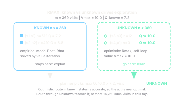
For known pairs, RMAX uses the empirical model $\hat{T}$ and $\hat{R}$ straight from the counts. For unknown pairs, it substitutes the rosiest possible model: reward $R_{\max}$ on every step plus a self loop, which gives value $V_{\max} = R_{\max} / (1 - \gamma)$ . It then runs value iteration on this optimistic model, acts greedily, updates counts after each real transition, and replans whenever a pair flips from unknown to known.

Now the neat either-or. If the optimistic plan stays inside known states, the simulation idea applies: an accurate model gives near-accurate values, with error growing as the horizon $1/(1 - \gamma)$ compounds. So the greedy act is near optimal and you exploited. If the optimistic plan reaches through an unknown, the agent walks there and collects the visits that make it known. You explored, and unknowns strictly shrink. Since there are only $S \times A$ pairs and each needs at most $m$ visits, unknown visits run out. The rest is bounding the small leaks, like acting on a known model that is still slightly off.

The trade is explicit. You pay up to $S \times A \times m$ exploratory visits for a guarantee that the remaining behavior is near optimal. The assumption is finite states and actions with bounded rewards and a fixed model. When states are huge or continuous, raw counts stop working and you need structure plus a different analysis. Then reach for function approximation tools, not a bigger $m$ .

Worked example: how many visits make a pair known?

Take a toy with $S = 10$ states and $A = 4$ actions, so $S \times A = 40$ pairs. Ask for reward accuracy $\alpha = 0.1$ per pair with overall confidence $\delta = 0.05$ . Rewards sit in $[0, 1]$ . This is the counting idea inside RMAX, simplified to one reward mean so you can check every digit. The full algorithm uses a larger $m$ because transition errors across $S$ outcomes compound through the horizon. Treat 369 as the illustration, not the deploy constant.

Split the failure budget evenly. Per-pair budget $\delta' = \delta / 40 = 0.00125$ . Hoeffding for a bounded mean says:

$P(|\hat{r} - r| \ge \alpha) \le 2 \exp(-2 m \alpha^2)$

Set the right side to $\delta'$ and solve:

$m \ge \frac{\ln(2 / \delta')}{2 \alpha^2}$

Plug in. $2 / 0.00125 = 1600$ . $\ln(1600) = 7.3778$ . Denominator $2 \times 0.01 = 0.02$ . Ratio $7.3778 / 0.02 = 368.8879$ . Round up, because visits are whole:

$m = 369$

After 369 visits to a pair, its reward estimate sits within 0.1 except with probability at most 0.05 spread across all 40 pairs. Pigeonhole next: at most $40 \times 369 = 14{,}760$ visits can land on unknowns before every pair turns known.

Now optimism picks the action. Set $R_{\max} = 1$ and $\gamma = 0.9$ , so $V_{\max} = 1 / (1 - 0.9) = 10.0$ . Suppose the best known pair offers $Q = 7.2$ while an unknown offers the optimistic $10.0$ . Ten beats seven point two, so the planner sends the agent to the unknown. Either the unknown delivers and you found something better, or its estimate falls after a few visits. Both outcomes are progress. The diagram draws exactly this split, and the code below recomputes both numbers.

How is this different from regret?

Regret adds up gaps: $\sum_t (V^{\ast}(s_t) - V^{A_t}(s_t))$ over $T$ steps. PAC-MDP counts bad steps: how many $t$ satisfy $V^{A_t}(s_t) < V^{\ast}(s_t) - \epsilon$ . Same run, different question. How much did you lose versus how often were you far off.

They connect through one safe split. Mistake steps lose at most $V_{\max}$ each, the rest lose at most $\epsilon$ each, so total regret is at most $N \times V_{\max} + T \times \epsilon$ where $N$ is the mistake count. But the two bars reward different behavior. Many tiny errors look bad to PAC with small $\epsilon$ yet cost little regret. A few huge exploration losses look fine to PAC yet hurt regret. Keep them apart. If you want the regret-flavored view of dithering versus bonuses, the exploration vs exploitation page centers it. If you want the model-free counterpart that later earned its own PAC result through delayed updates, read Q-learning.

Code

The snippet recomputes the threshold and the optimistic pick. It is deliberately small so you can rerun it.

1import math2
3
4def known_threshold(num_pairs: int, alpha: float, delta: float) -> int:5    per_pair: float = delta / num_pairs6    return math.ceil(math.log(2.0 / per_pair) / (2.0 * alpha * alpha))7
8
9def optimistic_value(r_max: float, gamma: float) -> float:10    return r_max / (1.0 - gamma)11
12
13m = known_threshold(40, 0.1, 0.05)14v_max = optimistic_value(1.0, 0.9)15q_known = 7.216choice = "unknown" if v_max > q_known else "known"17print(f"m = {m}")18print(f"Vmax = {v_max:.1f}")19print(f"Q_known = {q_known:.1f} -> pick {choice}")20assert m == 36921assert math.isclose(v_max, 10.0)22print("checks passed")

1# -> expected output:2m = 3693Vmax = 10.04Q_known = 7.2 -> pick unknown5checks passed

Watch Out For

PAC does not mean zero mistakes

Newcomers ship an optimistic learner and file a bug when early returns dip. That dip is the mechanism working. PAC allows a polynomial batch of $\epsilon$ -bad steps while the model fills in. In the toy above, up to 14,760 visits can hit unknowns before the partition closes, and those steps may look bad one by one.

The fix: test the right thing. Count $\epsilon$ -bad steps over long runs instead of demanding a clean first episode. If the count keeps growing past your budget as you scale $S$ or shrink $\epsilon$ , your $m$ or your planner is wrong, not the definition.

Delta is confidence, not accuracy

Readers see $1 - \delta = 95\%$ and hear within five percent of optimal. No. Epsilon is accuracy, how close the values must be. Delta is confidence over random runs, how often the bound holds. They move differently too. Halving $\alpha$ in the Hoeffding slice roughly quadruples $m$ because $\alpha^2$ sits in the denominator, while shrinking $\delta$ only grows $m$ logarithmically through $\ln(2/\delta')$ .

The fix: recompute $m$ when the setting changes. The 369 above belongs to $S = 10$ , $A = 4$ , $\alpha = 0.1$ , $\delta = 0.05$ . New sizes, new accuracy, or a transition-aware analysis all need their own arithmetic. Never paste 369 as a universal constant.

The Quick Version

PAC-MDP counts steps where the agent trails the optimum by more than epsilon, and calls learning efficient when that count stays polynomial in states, actions, accuracy, confidence, and horizon.
RMAX marks a state-action pair known after m visits, fits an empirical model there, and assigns maximum value to everything still unknown.
Unknown values of Vmax pull the planner toward novelty, so each plan either exploits an accurate known region or visits an unknown and shrinks that region.
Regret totals lost value across steps while PAC-MDP counts far-from-optimal steps, so one view prices exploration and the other rations it.
The toy threshold m equals 369 visits for 10 states, 4 actions, accuracy 0.1, and confidence 0.05, with Vmax 10 beating a known 7.2 to force one useful visit.