Policy Evaluation
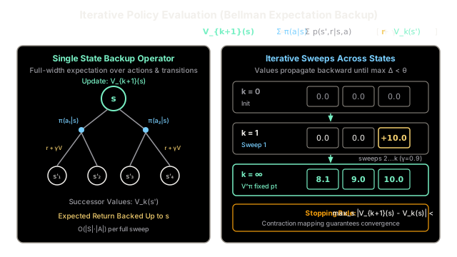
Iterative policy evaluation determines the true expected value of every state under a fixed policy by repeatedly applying Bellman backups until estimates converge.
Why Does This Exist?
In reinforcement learning, an agent cannot systematically improve its behavior without knowing the exact long-term return its current behavior produces. If an agent modifies its decisions arbitrarily without a reliable baseline, it risks choosing actions that yield immediate gratification but precipitate catastrophic long-term failure. Policy evaluation solves this foundational problem by computing the state-value function —the expected discounted cumulative reward from every state when following a specified policy .
Without policy evaluation, the foundational paradigm of Generalized Policy Iteration (GPI) breaks down. An agent must evaluate where it currently stands before it can identify which actions are genuinely superior.
Policy evaluation occupies a specific theoretical niche distinguishable from neighboring techniques:
- Versus Value Iteration: Value iteration computes the optimal value function directly by embedding a greedy policy maximization operator () into every single update sweep. Policy evaluation, by contrast, evaluates an arbitrary, fixed policy using the expectation over actions , decoupling evaluation from policy improvement.
- Versus Monte Carlo Evaluation: Monte Carlo methods estimate values by simulating sample trajectories until terminal episodes, requiring zero knowledge of environment transition dynamics but suffering from high sampling variance and failing on non-terminating horizons. Policy evaluation leverages full dynamic programming models to compute exact expectations across all branching paths in single-step sweeps with zero sample variance.
- Versus Temporal Difference (TD) Learning: TD methods update online from single observed state-action transitions , whereas dynamic programming policy evaluation performs an exhaustive, full-width expectation backup across all possible transitions simultaneously.
Think of It Like This
An Auditor Appraising a Fixed Corporate Business Plan
Imagine a senior financial auditor contracted to calculate the valuation of an enterprise operating under a rigid, unalterable business plan (the fixed policy ). The company sells recurring subscriptions with known retention rates, standard billing tiers, and fixed customer renewal discounts.
The auditor is strictly forbidden from changing business operations—they cannot adjust retail prices, alter marketing spend, or fire underperforming teams. Their sole mandate is to determine what every client account tier (state ) is worth across the total life of the contract.
- Initial ledger (): The auditor starts with a blank valuation sheet, initializing every customer account value to zero.
- First reconciliation sweep (): The auditor records only the immediate quarterly retainer fees billed today (immediate rewards ). Accounts that bill today show positive revenue; accounts that bill later remain zero.
- Compounding subsequent sweeps (): The auditor recognizes that retaining an account today guarantees a specific probability of renewal next quarter. They discount next quarter's revenue by an annual cost of capital and fold it into today's valuation sheet.
With each full audit cycle, valuation adjustments propagate backward through the client relationship pipeline. While early iterations produce large balance adjustments, the difference between consecutive audits eventually shrinks to pennies. Once the maximum adjustment across all account tiers drops below an auditing tolerance , the valuation ledger stabilizes into the true enterprise value .
The analogy stops because real economic markets face non-stationary macroeconomic shocks and unknown behavioral probabilities. Dynamic programming assumes stationary, fully modeled transition dynamics where every outcome probability is precisely specified.
How It Actually Works
The Bellman Expectation Backup and Contraction Mapping
Iterative policy evaluation operates on a Markov Decision Process (MDP) defined by the tuple , where is the finite set of states, is the action space, represents the environment dynamics, and is the discount factor.
For a fixed policy , the true state-value function satisfies the Bellman expectation equation:
When the state space is large, solving this system of linear equations directly via matrix inversion has time complexity , which quickly becomes prohibitive. Iterative policy evaluation turns this recursive equation into an iterative update rule. Starting with an arbitrary initial value vector (with ), the algorithm computes successive approximations:
Convergence is guaranteed by the Banach Fixed-Point Theorem. Defining the Bellman expectation operator as:
Under the supremum (infinity) norm , the operator satisfies:
Because , is a strict -contraction mapping on the complete metric space . This mathematical property guarantees:
- has a single, unique fixed point satisfying .
- The sequence generated by converges geometrically at rate to from any arbitrary initialization .
The iteration halts when the maximum change across all states between consecutive sweeps is strictly bounded by a small threshold :
By contraction properties, terminating at guarantees that the distance between the current estimate and the true value function satisfies:
Worked numerical example
Consider a 3-state linear Markov chain: leading to an absorbing terminal state where . The discount factor is , and the stopping threshold is .
Under policy , the agent transitions deterministically to the right:
- From , the agent steps to with reward .
- From , the agent steps to with reward .
- From , the agent steps into with reward .
Initialize all state values to zero at :
Iteration 1 ():
Compute the maximum update delta:
Since , the algorithm executes sweep 2 with value vector .
Iteration 2 ():
Compute the maximum update delta:
Since , values continue to propagate upstream with value vector .
Iteration 3 () and Final Convergence:
On iteration 4 (), evaluating all states yields identical values , producing . The iteration terminates at the exact analytical fixed point .
Code
from typing import List, Tuple
def iterative_policy_evaluation( grid_size: Tuple[int, int] = (4, 4), terminals: List[Tuple[int, int]] = [(0, 0), (3, 3)], gamma: float = 1.0, theta: float = 1e-4,) -> Tuple[List[List[float]], int]: """Computes state values for an equiprobable random policy on a Gridworld. Args: grid_size: Dimensions of the grid (rows, columns). terminals: List of coordinate tuples marking terminal states. gamma: Discount factor in [0, 1]. theta: Precision threshold for stopping condition. Returns: Tuple containing the converged 2D value grid and the iteration count. """ rows, cols = grid_size # Initialize state values to zero V: List[List[float]] = [[0.0 for _ in range(cols)] for _ in range(rows)] # Actions: Up, Down, Left, Right actions: List[Tuple[int, int]] = [(-1, 0), (1, 0), (0, -1), (0, 1)] prob_a: float = 1.0 / len(actions) iterations: int = 0
while True: delta: float = 0.0 # Create a copy for synchronous value updates new_V: List[List[float]] = [row[:] for row in V]
for r in range(rows): for c in range(cols): if (r, c) in terminals: continue
v_expected: float = 0.0 for dr, dc in actions: nr, nc = r + dr, c + dc # Wall bounce: staying in place if move goes off grid if not (0 <= nr < rows and 0 <= nc < cols): nr, nc = r, c reward: float = -1.0 v_expected += prob_a * (reward + gamma * V[nr][nc])
new_V[r][c] = v_expected delta = max(delta, abs(new_V[r][c] - V[r][c]))
V = new_V iterations += 1
if delta < theta: break
return V, iterations
if __name__ == "__main__": converged_V, num_sweeps = iterative_policy_evaluation() print(f"Converged after {num_sweeps} sweeps:") for row in converged_V: print([round(val, 1) for val in row])
# Expected output: # Converged after 173 sweeps: # [0.0, -14.0, -20.0, -22.0] # [-14.0, -18.0, -20.0, -20.0] # [-20.0, -20.0, -18.0, -14.0] # [-22.0, -20.0, -14.0, 0.0]Watch Out For
Stopping Threshold Pitfall: Incomplete Convergence vs Excessive Computation
Setting the convergence threshold creates a sharp trade-off between numerical precision and computational waste:
- Stopping Too Early ( too loose): In policy evaluation, reward information propagates backward only one transition step per sweep. If is set too large (e.g., ), the algorithm halts before value signals from distant rewards reach early upstream states. In Generalized Policy Iteration, acting greedily on half-propagated value estimates causes the policy improvement step to select suboptimal actions.
- Stopping Too Late ( excessively tight): Because convergence is asymptotic, setting forces dozens of costly sweeps computing negligible micro-adjustments that have zero influence on which action has the highest value.
- The Fix: Bound the true value error using the theoretical relation . If using policy evaluation inside Policy Iteration, truncate policy evaluation early: truncating after just 5 to 10 sweeps (as done in Value Iteration or Modified Policy Iteration) still guarantees policy improvement while slashing computation by orders of magnitude.
The Quick Version
- Policy evaluation computes the true state-value function for an unvarying policy without modifying agent decisions.
- It iteratively applies the Bellman expectation backup operator across all states: .
- Because the Bellman expectation operator is a contraction mapping in the infinity norm, convergence to a unique fixed point is guaranteed for any initial values when .
- The sweep loop terminates once the maximum single-state variation falls below a specified tolerance threshold .