Policy Improvement

Policy improvement transforms an existing policy into a superior one by choosing actions that maximize expected return under current value estimates.

Why Does This Exist?

In reinforcement learning, evaluating an agent's current strategy through policy evaluation computes how much cumulative return each state yields under that fixed behavior. However, evaluation alone does not change behavior. To discover an optimal strategy, an agent requires a systematic, mathematically principled mechanism to upgrade its choices.

Without a formal improvement rule, attempting to modify an agent's actions risks catastrophic instability. In a sequential decision problem, changing an action in one state alters the state distribution and downstream trajectories throughout the entire environment. Naively tweaking actions can inadvertently degrade long-term performance, trap the agent in suboptimal cycles, or cause performance collapse.

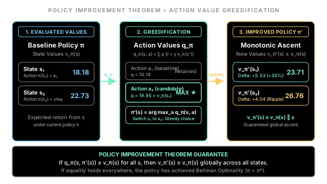
The Policy Improvement Theorem provides the theoretical guarantee that prevents this failure. It proves that by taking an action that looks locally greedy with respect to the current state-value function $v_\pi$ , the resulting policy $\pi'$ is guaranteed to achieve equal or greater expected return from every single state in the environment ( $v_{\pi'}(s) \ge v_\pi(s)$ for all $s$ ). This monotonic improvement property turns policy search into an orderly ascent toward optimality.

Think of It Like This

Upgrading Chess Openings Against an Opponent's Repertoire

Imagine you are a tournament chess player with an established opening repertoire ( $\pi$ ). After analyzing hundreds of recorded games against a rival, your chess engine calculates your expected win rate from every board position that typically arises ( $v_\pi(s)$ ).

On move 6, your traditional opening book dictates playing a modest pawn move $a_1$ . Your engine evaluation shows that $a_1$ maintains your baseline win expectation of $+0.20$ ( $v_\pi(s) = 0.20$ ). However, deep engine calculations reveal an alternative knight move $a_2$ : taking this move yields an immediate tactical threat and leads to board configurations that evaluate to $+0.80$ ( $q_\pi(s, a_2) = 0.80$ ), even assuming you revert to your standard opening repertoire for all subsequent moves.

Policy improvement is the decision to update your opening notebook: whenever you reach this specific board state, you permanently replace $a_1$ with $a_2$ ( $\pi'(s) = a_2$ ).

Because the expected return of taking $a_2$ once and following $\pi$ thereafter exceeds the baseline value of $\pi$ , committing to $a_2$ every time you encounter that position can never hurt your long-term score. Even better, because this superior position is reached repeatedly, the advantage compounds across all subsequent games.

Where the analogy stops: In tournament chess, a human opponent actively studies your games and prepares counter-strategies in response, creating a non-stationary two-player game. In a standard Markov Decision Process, the environment's transition dynamics and reward functions remain stationary, meaning that improvements against the environment never trigger an adversarial counter-adjustment.

How It Actually Works

Action-Value Greedification and the Policy Improvement Theorem

Let an environment be defined as a Markov Decision Process $(\mathcal{S}, \mathcal{A}, p, \gamma)$ , where $\mathcal{S}$ is the state space, $\mathcal{A}$ is the action space, $p(s', r \mid s, a)$ represents the transition dynamics, and $\gamma \in [0, 1)$ is the discount factor.

Suppose the agent follows an initial deterministic policy $\pi: \mathcal{S} \to \mathcal{A}$ , yielding evaluated state-values $v_\pi(s) = \mathbb{E}_\pi [G_t \mid S_t = s]$ .

1. Computing Action-Values

To determine whether selecting an alternative action $a \neq \pi(s)$ in state $s$ improves return, we evaluate the action-value function $q_\pi(s, a)$ . This represents the expected return of taking action $a$ right now, and subsequently following policy $\pi$ forever after:

q_\pi(s, a) \doteq \mathbb{E}_\pi [R_{t+1} + \gamma v_\pi(S_{t+1}) \mid S_t = s, A_t = a] = \sum_{s' \in \mathcal{S}} \sum_{r \in \mathcal{R}} p(s', r \mid s, a) \left[ r + \gamma v_\pi(s') \right]

2. Greedification (Policy Update)

We construct a new deterministic policy $\pi'$ by selecting the action that maximizes $q_\pi(s, a)$ at each state:

\pi'(s) \doteq \arg\max_{a \in \mathcal{A}} q_\pi(s, a) = \arg\max_{a \in \mathcal{A}} \sum_{s', r} p(s', r \mid s, a) \left[ r + \gamma v_\pi(s') \right]

By definition of the $\arg\max$ operator, the new action satisfies:

q_\pi(s, \pi'(s)) = \max_{a \in \mathcal{A}} q_\pi(s, a) \ge q_\pi(s, \pi(s)) = v_\pi(s)

3. Mathematical Proof of the Policy Improvement Theorem

The Policy Improvement Theorem (Bellman, 1957; Howard, 1960; Sutton & Barto, 2018) asserts:

If $q_\pi(s, \pi'(s)) \ge v_\pi(s)$ for all $s \in \mathcal{S}$ , then the overall policy $\pi'$ is globally as good as, or better than, $\pi$ : $v_{\pi'}(s) \ge v_\pi(s) \quad \forall s \in \mathcal{S}$

The proof proceeds by repeatedly unrolling the Bellman inequality:

\begin{aligned} v_\pi(s) &\le q_\pi(s, \pi'(s)) \\ &= \mathbb{E}[R_{t+1} + \gamma v_\pi(S_{t+1}) \mid S_t = s, A_t = \pi'(s)] \\ &= \mathbb{E}_{\pi'}[R_{t+1} + \gamma v_\pi(S_{t+1}) \mid S_t = s] \end{aligned}

Because the inequality $v_\pi(s') \le q_\pi(s', \pi'(s'))$ holds for every successor state $s'$ , we substitute $v_\pi(S_{t+1}) \le \mathbb{E}_{\pi'}[R_{t+2} + \gamma v_\pi(S_{t+2}) \mid S_{t+1}]$ into the expression:

\begin{aligned} v_\pi(s) &\le \mathbb{E}_{\pi'}[R_{t+1} + \gamma \mathbb{E}_{\pi'}[R_{t+2} + \gamma v_\pi(S_{t+2}) \mid S_{t+1}] \mid S_t = s] \\ &= \mathbb{E}_{\pi'}[R_{t+1} + \gamma R_{t+2} + \gamma^2 v_\pi(S_{t+2}) \mid S_t = s] \end{aligned}

Expanding this relationship recursively across $k$ consecutive time steps:

v_\pi(s) \le \mathbb{E}_{\pi'}\left[ R_{t+1} + \gamma R_{t+2} + \gamma^2 R_{t+3} + \dots + \gamma^{k-1} R_{t+k} + \gamma^k v_\pi(S_{t+k}) \,\middle|\, S_t = s \right]

Taking the infinite-horizon limit as $k \to \infty$ , with discount factor $\gamma < 1$ and bounded immediate rewards, the terminal discounted term vanishes: $\lim_{k \to \infty} \gamma^k \mathbb{E}_{\pi'}[v_\pi(S_{t+k})] = 0$ . Therefore:

v_\pi(s) \le \mathbb{E}_{\pi'}\left[ \sum_{k=0}^{\infty} \gamma^k R_{t+k+1} \,\middle|\, S_t = s \right] = v_{\pi'}(s)

This completes the proof: $v_{\pi'}(s) \ge v_\pi(s)$ for all $s \in \mathcal{S}$ .

4. Convergence to Optimality

If the improved policy $\pi'$ achieves strictly identical values to $\pi$ ( $v_{\pi'}(s) = v_\pi(s)$ for all $s$ ), then:

v_{\pi'}(s) = \max_{a \in \mathcal{A}} \sum_{s', r} p(s', r \mid s, a) \left[ r + \gamma v_{\pi'}(s') \right]

This matches the Bellman Optimality Equation. Consequently, both $\pi$ and $\pi'$ must be optimal policies $\pi^*$ . In any finite MDP with $|\mathcal{S}|$ states and $|\mathcal{A}|$ actions, there are exactly $|\mathcal{A}|^{|\mathcal{S}|}$ distinct deterministic policies; because each improvement step strictly increases value until reaching optimality, policy improvement cannot cycle and must terminate at the optimal policy in a finite number of steps.

Worked numerical example

Consider a 2-state environment with discount factor $\gamma = 0.90$ :

State $s_1$ $s_{1}$ (Staging Area) offers two actions:
- $a_1$ (Conservative): Transitions to $s_1$ with probability $0.80$ ( $r = +1.0$ ), and to $s_2$ with probability $0.20$ ( $r = +1.0$ ).
- $a_2$ (Venturesome): Transitions to $s_2$ with probability $0.90$ ( $r = 0.0$ ), and slips back to $s_1$ with probability $0.10$ ( $r = -1.0$ ).
State $s_2$ $s_{2}$ (High-Yield Vault) has a single fixed action:
- $\text{stay}$ : Transitions to $s_2$ with probability $0.70$ ( $r = +5.0$ ), and drops back to $s_1$ with probability $0.30$ ( $r = 0.0$ ).

Step 1: Evaluate Baseline Policy $\pi$

Our baseline policy $\pi$ selects action $a_1$ in $s_1$ ( $\pi(s_1) = a_1$ ). We solve the linear Bellman expectation system:

\begin{aligned} v_\pi(s_1) &= 0.80 [1.0 + 0.90 v_\pi(s_1)] + 0.20 [1.0 + 0.90 v_\pi(s_2)] = 1.00 + 0.72 v_\pi(s_1) + 0.18 v_\pi(s_2) \\ v_\pi(s_2) &= 0.70 [5.0 + 0.90 v_\pi(s_2)] + 0.30 [0.0 + 0.90 v_\pi(s_1)] = 3.50 + 0.63 v_\pi(s_2) + 0.27 v_\pi(s_1) \end{aligned}

Rearranging into standard matrix form:

\begin{bmatrix} 0.28 & -0.18 \\ -0.27 & 0.37 \end{bmatrix} \begin{bmatrix} v_\pi(s_1) \\ v_\pi(s_2) \end{bmatrix} = \begin{bmatrix} 1.00 \\ 3.50 \end{bmatrix}

Solving this system yields:

v_\pi(s_1) \approx 18.18, \qquad v_\pi(s_2) \approx 22.73

Step 2: Compute Action-Values $q_\pi(s_1, a)$

Now we evaluate both candidate actions available in state $s_1$ :

Action $a_1$ : $q_\pi(s_1, a_1) = 1.00 + 0.72(18.18) + 0.18(22.73) = 18.18 = v_\pi(s_1)$
Action $a_2$ : $\begin{aligned} q_\pi(s_1, a_2) &= 0.90 [0.0 + 0.90 \times v_\pi(s_2)] + 0.10 [-1.0 + 0.90 \times v_\pi(s_1)] \\ &= 0.90 [0.90 \times 22.73] + 0.10 [-1.0 + 0.90 \times 18.18] \\ &= 0.90 [20.457] + 0.10 [15.362] \\ &= 18.411 + 1.536 = 19.95 \end{aligned}$

Comparing the two action-values:

q_\pi(s_1, a_2) = 19.95 > v_\pi(s_1) = 18.18

Step 3: Greedification

The policy improvement step selects:

\pi'(s_1) = \arg\max_{a \in \{a_1, a_2\}} q_\pi(s_1, a) = a_2

Step 4: True Value of the Improved Policy $\pi'$

Now we compute the actual state values $v_{\pi'}$ under the updated policy:

\begin{aligned} v_{\pi'}(s_1) &= 0.10 [-1.0 + 0.90 v_{\pi'}(s_1)] + 0.90 [0.0 + 0.90 v_{\pi'}(s_2)] = -0.10 + 0.09 v_{\pi'}(s_1) + 0.81 v_{\pi'}(s_2) \\ v_{\pi'}(s_2) &= 3.50 + 0.63 v_{\pi'}(s_2) + 0.27 v_{\pi'}(s_1) \end{aligned}

In matrix form:

\begin{bmatrix} 0.91 & -0.81 \\ -0.27 & 0.37 \end{bmatrix} \begin{bmatrix} v_{\pi'}(s_1) \\ v_{\pi'}(s_2) \end{bmatrix} = \begin{bmatrix} -0.10 \\ 3.50 \end{bmatrix}

Solving this linear system gives:

v_{\pi'}(s_1) \approx 23.71, \qquad v_{\pi'}(s_2) \approx 26.76

Notice the global ripple effect:

$v_{\pi'}(s_1) - v_\pi(s_1) = 23.71 - 18.18 = +5.53$ (+30.4% gain)
$v_{\pi'}(s_2) - v_\pi(s_2) = 26.76 - 22.73 = +4.03$ (+17.7% gain)

Even though the agent took the exact same action in state $s_2$ , its value rose by $+4.03$ because when transitions occasionally drop the agent back into $s_1$ , the improved policy makes the superior choice $a_2$ , boosting cumulative returns across the entire trajectory.

Code

1from typing import Dict, List, Tuple2
3# Transition model: (state, action) -> list of (probability, next_state, reward)4TransitionModel = Dict[Tuple[str, str], List[Tuple[float, str, float]]]5Policy = Dict[str, str]6ValueFunction = Dict[str, float]7
8
9def evaluate_policy(10    policy: Policy,11    transitions: TransitionModel,12    states: List[str],13    gamma: float = 0.9,14    theta: float = 1e-9,15) -> ValueFunction:16    """Iteratively computes state values v_pi(s) via the Bellman expectation equation."""17    v: ValueFunction = {s: 0.0 for s in states}18    while True:19        delta = 0.020        for s in states:21            a = policy[s]22            # Bellman expectation backup: v(s) = sum_{s', r} p(s', r | s, a) * [r + gamma * v(s')]23            v_new = sum(24                prob * (r + gamma * v[s_next])25                for prob, s_next, r in transitions[(s, a)]26            )27            delta = max(delta, abs(v[s] - v_new))28            v[s] = v_new29        if delta < theta:30            break31    return v32
33
34def compute_action_value(35    state: str,36    action: str,37    v: ValueFunction,38    transitions: TransitionModel,39    gamma: float = 0.9,40) -> float:41    """Computes q_pi(s, a) = sum_{s', r} p(s', r | s, a) * [r + gamma * v(s')]."""42    return sum(43        prob * (r + gamma * v[s_next])44        for prob, s_next, r in transitions[(state, action)]45    )46
47
48def policy_improvement(49    v: ValueFunction,50    transitions: TransitionModel,51    states: List[str],52    actions: Dict[str, List[str]],53    gamma: float = 0.9,54) -> Policy:55    """56    Greedifies policy: pi'(s) = argmax_a q_pi(s, a).57    Applies deterministic tie-breaking by candidate order.58    """59    improved_policy: Policy = {}60
61    for s in states:62        available_actions = actions[s]63        # Evaluate q_pi(s, a) for all candidate actions64        action_values = {65            a: compute_action_value(s, a, v, transitions, gamma)66            for a in available_actions67        }68        # Deterministic greedification: break numerical ties by fixed index69        best_action = max(70            available_actions,71            key=lambda a: (round(action_values[a], 7), -available_actions.index(a)),72        )73        improved_policy[s] = best_action74
75    return improved_policy76
77
78if __name__ == "__main__":79    states = ["s1", "s2"]80    actions = {81        "s1": ["a1", "a2"],82        "s2": ["stay"],83    }84    transitions: TransitionModel = {85        ("s1", "a1"): [(0.8, "s1", 1.0), (0.2, "s2", 1.0)],86        ("s1", "a2"): [(0.9, "s2", 0.0), (0.1, "s1", -1.0)],87        ("s2", "stay"): [(0.7, "s2", 5.0), (0.3, "s1", 0.0)],88    }89    gamma = 0.990
91    # 1. Evaluate baseline policy pi where pi(s1) = a192    baseline_policy: Policy = {"s1": "a1", "s2": "stay"}93    v_pi = evaluate_policy(baseline_policy, transitions, states, gamma=gamma)94
95    print("--- 1. Baseline Policy Evaluation v_pi ---")96    for s in states:97        print(f"v_pi({s}) = {v_pi[s]:.2f}")98
99    # 2. Compute action-values q_pi(s1, a)100    print("\n--- 2. Action-Value Greedification in s1 ---")101    q_s1_a1 = compute_action_value("s1", "a1", v_pi, transitions, gamma=gamma)102    q_s1_a2 = compute_action_value("s1", "a2", v_pi, transitions, gamma=gamma)103    print(f"q_pi(s1, a1) = {q_s1_a1:.2f} (current baseline)")104    print(f"q_pi(s1, a2) = {q_s1_a2:.2f} (candidate improvement)")105
106    # 3. Policy improvement step107    improved_policy = policy_improvement(v_pi, transitions, states, actions, gamma=gamma)108    print(f"\nImproved Policy pi': {improved_policy}")109
110    # 4. Evaluate new policy pi'111    v_prime = evaluate_policy(improved_policy, transitions, states, gamma=gamma)112    print("\n--- 3. Improved Policy Evaluation v_pi' ---")113    for s in states:114        print(f"v_pi'({s}) = {v_prime[s]:.2f} (Delta: +{v_prime[s] - v_pi[s]:.2f})")115
116    # Assertions validating Policy Improvement Theorem117    assert q_s1_a2 > v_pi["s1"], "Candidate action must yield strictly higher q-value"118    assert improved_policy["s1"] == "a2", "Greedy update must select action a2"119    assert v_prime["s1"] >= v_pi["s1"], "Monotonic improvement guarantee violated for s1"120    assert v_prime["s2"] >= v_pi["s2"], "Monotonic improvement guarantee violated for s2"121    print("\nPolicy Improvement Theorem assertions passed successfully.")

1--- 1. Baseline Policy Evaluation v_pi ---2v_pi(s1) = 18.183v_pi(s2) = 22.734
5--- 2. Action-Value Greedification in s1 ---6q_pi(s1, a1) = 18.18 (current baseline)7q_pi(s1, a2) = 19.95 (candidate improvement)8
9Improved Policy pi': {'s1': 'a2', 's2': 'stay'}10
11--- 3. Improved Policy Evaluation v_pi' ---12v_pi'(s1) = 23.71 (Delta: +5.53)13v_pi'(s2) = 26.76 (Delta: +4.04)14
15Policy Improvement Theorem assertions passed successfully.

Watch Out For

Non-deterministic tie-breaking causing policy oscillation

When two or more actions yield identical action-values ( $q_\pi(s, a_1) = q_\pi(s, a_2)$ ), arbitrary or random tie-breaking breaks convergence. If Python's dictionary iteration or non-deterministic sorting flips the winner on consecutive iterations, policy iteration will oscillate endlessly between $a_1$ and $a_2$ despite having already reached optimal value.

Symptom: The policy never stabilizes, reporting changes on every iteration even though state values have completely converged ( $\Delta v = 0$ ).

Fix: Implement a strict, deterministic tie-breaking rule. Always prefer retaining the existing action $\pi(s)$ whenever an alternative action's value is within numerical tolerance $|q(s, a) - q(s, \pi(s))| \le 10^{-7}$ . If multiple novel actions tie, break ties using a fixed alphabetical or indexed action hierarchy.

Greedifying on imprecise or noisy value estimates

The Policy Improvement Theorem strictly guarantees $v_{\pi'}(s) \ge v_\pi(s)$ only when action-values are computed from the exact true state values $v_\pi$ . In approximate reinforcement learning or early-stopped policy evaluation, value estimates contain estimation errors $\hat{v}_\pi = v_\pi + \epsilon$ .

Symptom: Greedification on noisy value estimates selects an action that appears superficially better but actually degrades policy return ( $v_{\pi'}(s) < v_\pi(s)$ ), causing policy degradation or divergence.

Fix: In dynamic programming, ensure iterative policy evaluation converges beneath a stringent threshold ( $\theta \le 10^{-8}$ ) before greedifying. In sample-based or deep reinforcement learning, avoid hard 1-step greedification; instead, employ conservative policy updates, trust-region constraints (such as TRPO or PPO), or entropy-regularized policy gradients that bound policy divergence per step.

The Quick Version

Policy improvement generates a new policy $\pi'$ by acting greedily with respect to current value estimates: $\pi'(s) = \arg\max_a q_\pi(s, a)$ .
The Policy Improvement Theorem mathematically guarantees monotonic non-decreasing expected return from every state: $v_{\pi'}(s) \ge v_\pi(s)$ for all $s \in \mathcal{S}$ .
Greedifying an action in one state causes a positive ripple effect throughout the entire Markov chain, increasing values even in states where the policy did not change.
When greedification produces no change in policy return ( $v_{\pi'}(s) = v_\pi(s)$ for all $s$ ), the policy has satisfied the Bellman Optimality Equation and is guaranteed optimal ( $\pi = \pi^*$ ).