Polynomials and Fourier Basis in RL

Instead of struggling to fit complex value landscapes with unstable polynomial curves, the Fourier basis decomposes continuous states into harmonious, orthogonal cosine waves of increasing frequency.

Comparing polynomial basis functions with the bounded, orthogonal Fourier cosine basis for linear value function approximation in continuous state spaces.

Why Does This Exist?

When reinforcement learning moves from discrete gridworlds to continuous physical systems—such as controlling a robot arm, balancing a cart-pole, or piloting a spacecraft—tabular Q-learning breaks down because the number of distinct states is infinite. The agent must approximate value functions using function approximation:

$\hat{v}(\mathbf{s}, \mathbf{w}) = \mathbf{w}^\top \boldsymbol{\phi}(\mathbf{s})$

Where $\boldsymbol{\phi}(\mathbf{s})$ is a feature vector that transforms raw continuous state coordinates $\mathbf{s} \in \mathbb{R}^k$ into a higher-dimensional space where linear methods can represent non-linear value surfaces.

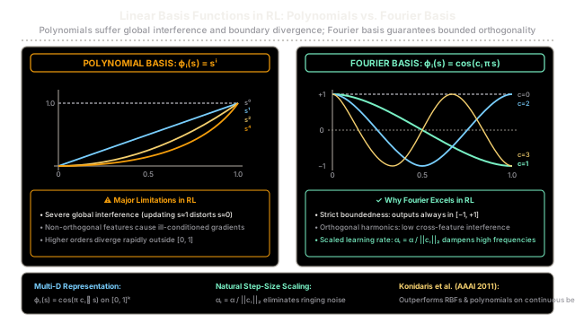
The most naive feature transformation is the polynomial basis, constructing features from powers and cross-products ( $1, s_1, s_2, s_1 s_2, s_1^2, \dots$ ). While mathematically straightforward, polynomials suffer from fatal pathologies in reinforcement learning:

Global interference: A temporal difference error observed in one corner of the state space modifies polynomial weights that warp value predictions everywhere else, causing catastrophic forgetting.
Runge's phenomenon and unbounded divergence: Higher-order polynomial features shoot toward $\pm \infty$ near the boundaries of the state space, making gradient updates violently unstable.
Ill-conditioned Hessians: Polynomial features are non-orthogonal, causing gradient descent to oscillate erratically across narrow error valleys.

To overcome these structural flaws, George Konidaris, Sarah Osentoski, and Philip Thomas (2011) introduced the Fourier basis for reinforcement learning. By using orthogonal cosine harmonics over a normalized hypercube $[0, 1]^k$ , the Fourier basis guarantees bounded feature outputs in $[-1, 1]$ , eliminates destructive global interference, and provides a mathematically grounded frequency-dependent learning rate rule that outperforms polynomials and radial basis functions across continuous control benchmarks.

Think of It Like This

Musical Synthesizers: Taylor Series Polynomials vs. Fourier Harmonic Overtones

Imagine trying to synthesize the warm acoustic resonance of a concert cello on an electronic keyboard:

The Polynomial Approach (Brute-Force Taylor Approximation): You try to craft the cello's sound wave by superimposing steep algebraic powers: $x, x^2, x^3, x^4, x^5$ . Because high powers shoot off to infinity at the edges, turning up the volume on $x^5$ to fix a tiny buzzing artifact at the end of the note completely destroys the pitch in the middle of the wave. The entire keyboard screeches with wild, unpredictable distortion.
The Fourier Basis Approach (Harmonic Synthesis): You synthesize the cello using pure sinusoidal harmonics. You start with the fundamental pitch (the low-frequency base tone, $\cos(\pi s)$ ), and then add subtle second, third, and fourth harmonic overtones of increasing frequency ( $\cos(2\pi s), \cos(3\pi s)$ ) at decreasing volumes. Because each harmonic is mathematically orthogonal, adjusting a high-frequency overtone adds fine musical texture without altering the fundamental pitch. The sound remains rich, stable, and perfectly bounded within the speaker's dynamic range.

Where the analogy stops: In sound synthesis, harmonics travel across continuous time. In reinforcement learning, the Fourier basis projects continuous spatial state vectors $\mathbf{s} \in [0, 1]^k$ onto multi-dimensional frequency vectors $\mathbf{c}_i \in \{0, \dots, n\}^k$ to approximate state values and action-value surfaces.

How It Actually Works

Polynomial Limitations and Konidaris' Fourier Cosine Basis

Consider a continuous state space of dimension $k$ , where the state vector is $\mathbf{s} = [s_1, s_2, \dots, s_k]^\top$ .

1. The Polynomial Basis

For an order- $n$ polynomial basis, each feature $\phi_i(\mathbf{s})$ is formed by integer exponents $c_{i, j} \in \{0, 1, \dots, n\}$ :

$\phi_i(\mathbf{s}) = \prod_{j=1}^k s_j^{c_{i, j}}$

For a 2D state space $\mathbf{s} = [s_1, s_2]^\top$ with order $n = 2$ , the complete basis consists of $(n+1)^k = 9$ features: $\boldsymbol{\phi}(\mathbf{s}) = \left[ 1, s_1, s_2, s_1^2, s_2^2, s_1 s_2, s_1^2 s_2, s_1 s_2^2, s_1^2 s_2^2 \right]^\top$

Because these features are not orthogonal over the state domain, their inner products are heavily coupled. Updating weight $w_i$ for $s_1^2$ alters values across the entire state space, making semi-gradient TD updates sluggish and prone to divergence.

2. The Fourier Cosine Basis

Konidaris et al. demonstrated that using only the cosine functions of a multidimensional Fourier series provides an exceptional basis for linear value approximation. Cosine functions are symmetric about the origin, naturally representing boundary conditions where derivative fluxes approach zero.

Before feature evaluation, continuous state coordinates must be normalized into the unit hypercube: $s_j \in [0, 1] \quad \forall j \in \{1, \dots, k\}$

For an order- $n$ Fourier basis, each basis feature $\phi_i(\mathbf{s})$ is defined by an integer coefficient vector $\mathbf{c}_i = [c_{i, 1}, c_{i, 2}, \dots, c_{i, k}]^\top$ with each $c_{i, j} \in \{0, 1, \dots, n\}$ :

$\phi_i(\mathbf{s}) = \cos\left( \pi \mathbf{c}_i^\top \mathbf{s} \right) = \cos\left( \pi \sum_{j=1}^k c_{i, j} s_j \right)$

The total number of basis features for an order- $n$ expansion in $k$ dimensions is $(n + 1)^k$ .

3. Why the Fourier Basis Excels in RL

The Fourier basis possesses three mathematical properties that make it uniquely suited for temporal difference learning:

Strict Boundedness: $\phi_i(\mathbf{s}) \in [-1, 1] \quad \forall \mathbf{s} \in [0, 1]^k$ Features cannot explode, preventing numerical overflow and gradient spikes.
Orthogonality: The basis functions form an orthogonal set under the $L^2$ inner product over $[0, 1]^k$ : $\int_{[0, 1]^k} \cos(\pi \mathbf{c}_i^\top \mathbf{s}) \cos(\pi \mathbf{c}_j^\top \mathbf{s}) \, d\mathbf{s} = 0 \quad \text{for } \mathbf{c}_i \ne \mathbf{c}_j$ This near-zero cross-correlation keeps the gradient covariance matrix well-conditioned, drastically reducing destructive interference between coarse and fine features.
The Natural Frequency-Scaled Step Size Rule: In Fourier analysis, the $L^2$ norm of the gradient scales with frequency $\|\mathbf{c}_i\|_2$ . Konidaris et al. proved that applying a uniform learning rate $\alpha$ causes high-frequency features to update too aggressively, producing severe high-frequency oscillations ("ringing").

To maintain uniform parameter convergence rates across all spatial scales, learning rates must be scaled inversely with the Euclidean norm of the coefficient vector: $\alpha_i = \begin{cases} \alpha & \text{if } \|\mathbf{c}_i\|_2 = 0 \\ \frac{\alpha}{\|\mathbf{c}_i\|_2} & \text{if } \|\mathbf{c}_i\|_2 > 0 \end{cases}$ Where $\|\mathbf{c}_i\|_2 = \sqrt{\sum_{j=1}^k c_{i, j}^2}$ .

This rule automatically lets low-frequency features capture broad value topography quickly, while high-frequency features gently refine localized details without instability.

Worked numerical example

Consider a 2D continuous state space (e.g., Mountain Car position and velocity) with order $n = 1$ .

Let:

Continuous state $\mathbf{s} = [0.2, 0.8]^\top \in [0, 1]^2$
Base learning rate $\alpha = 0.01$
Order $n = 1 \implies (1 + 1)^2 = 4$ basis vectors $\mathbf{c}_0, \dots, \mathbf{c}_3 \in \{0, 1\}^2$

Let us compute the features $\phi_i(\mathbf{s})$ and scaled learning rates $\alpha_i$ step by step:

1. Feature 0: Bias Term ( $\mathbf{c}_0 = [0, 0]^\top$ )

Frequency norm: $\|\mathbf{c}_0\|_2 = \sqrt{0^2 + 0^2} = 0.0$
Inner product: $\mathbf{c}_0^\top \mathbf{s} = 0(0.2) + 0(0.8) = 0.0$
Feature value: $\phi_0(\mathbf{s}) = \cos(\pi \times 0.0) = \mathbf{1.0000}$
Learning rate: $\alpha_0 = \alpha = \mathbf{0.0100}$

2. Feature 1: Variation along Dimension 2 ( $\mathbf{c}_1 = [0, 1]^\top$ )

Frequency norm: $\|\mathbf{c}_1\|_2 = \sqrt{0^2 + 1^2} = 1.0$
Inner product: $\mathbf{c}_1^\top \mathbf{s} = 0(0.2) + 1(0.8) = 0.8$
Feature value: $\phi_1(\mathbf{s}) = \cos(0.8 \pi) = \cos(144^\circ) = \mathbf{-0.8090}$
Learning rate: $\alpha_1 = \frac{0.01}{1.0} = \mathbf{0.0100}$

3. Feature 2: Variation along Dimension 1 ( $\mathbf{c}_2 = [1, 0]^\top$ )

Frequency norm: $\|\mathbf{c}_2\|_2 = \sqrt{1^2 + 0^2} = 1.0$
Inner product: $\mathbf{c}_2^\top \mathbf{s} = 1(0.2) + 0(0.8) = 0.2$
Feature value: $\phi_2(\mathbf{s}) = \cos(0.2 \pi) = \cos(36^\circ) = \mathbf{+0.8090}$
Learning rate: $\alpha_2 = \frac{0.01}{1.0} = \mathbf{0.0100}$

4. Feature 3: Coupled Diagonal Variation ( $\mathbf{c}_3 = [1, 1]^\top$ )

Frequency norm: $\|\mathbf{c}_3\|_2 = \sqrt{1^2 + 1^2} = \sqrt{2} \approx 1.4142$
Inner product: $\mathbf{c}_3^\top \mathbf{s} = 1(0.2) + 1(0.8) = 1.0$
Feature value: $\phi_3(\mathbf{s}) = \cos(1.0 \pi) = \cos(180^\circ) = \mathbf{-1.0000}$
Scaled learning rate: $\alpha_3 = \frac{0.01}{\sqrt{2}} = \frac{0.01}{1.4142} \approx \mathbf{0.007071}$

Summary Table

Index $i$	Frequency Vector $\mathbf{c}_i$	Frequency Norm $\\|\mathbf{c}_i\\|_2$	Feature $\phi_i(\mathbf{s})$	Scaled Step Size $\alpha_i$	Spatial Role
$0$	$[0, 0]^\top$	$0.0000$	$+1.0000$	$0.010000$	Baseline DC bias
$1$	$[0, 1]^\top$	$1.0000$	$-0.8090$	$0.010000$	Pure vertical axis mode
$2$	$[1, 0]^\top$	$1.0000$	$+0.8090$	$0.010000$	Pure horizontal axis mode
$3$	$[1, 1]^\top$	$1.4142$	$-1.0000$	$0.007071$	Coupled diagonal interaction

Notice how $\alpha_3$ is automatically damped by $30\%$ to ensure high-frequency cross-terms do not oscillate during value updates.

Code

The following complete, type-hinted Python implementation constructs a multi-dimensional Fourier basis encoder, precomputes frequency-scaled learning rates, and updates a linear value approximator with assertion checks.

1import itertools2import math3from typing import List, Tuple4
5
6class FourierBasis:7    """Fourier Cosine Basis linear feature encoder for continuous RL states.8
9    References:10        Konidaris, Osentoski, and Thomas (AAAI 2011).11        'Value Function Approximation in Reinforcement Learning using the Fourier Basis'12    """13
14    def __init__(15        self,16        state_dim: int,17        order: int,18        state_bounds: List[Tuple[float, float]],19        base_alpha: float = 0.01,20    ) -> None:21        self.state_dim: int = state_dim22        self.order: int = order23        self.state_bounds: List[Tuple[float, float]] = state_bounds24        self.base_alpha: float = base_alpha25
26        # Generate all multi-frequency coefficient vectors c in {0, ..., order}^k27        coord_ranges = [range(order + 1) for _ in range(state_dim)]28        self.c_vectors: List[List[int]] = [29            list(c) for c in itertools.product(*coord_ranges)30        ]31        self.num_features: int = len(self.c_vectors)32
33        # Precompute frequency-scaled step sizes: alpha_i = alpha / ||c_i||_234        self.alphas: List[float] = []35        for c in self.c_vectors:36            norm = math.sqrt(sum(ci**2 for ci in c))37            self.alphas.append(base_alpha if norm == 0 else base_alpha / norm)38
39        # Initialize linear weights vector to zero40        self.weights: List[float] = [0.0] * self.num_features41
42    def normalize_state(self, state: List[float]) -> List[float]:43        """Linearly projects continuous state into unit hypercube [0, 1]^k."""44        normalized: List[float] = []45        for s_val, (s_min, s_max) in zip(state, self.state_bounds):46            clamped = max(s_min, min(s_max, s_val))47            norm_val = (48                (clamped - s_min) / (s_max - s_min) if s_max > s_min else 0.049            )50            normalized.append(norm_val)51        return normalized52
53    def encode(self, state: List[float]) -> List[float]:54        """Computes basis features phi_i(s) = cos(pi * c_i^T s)."""55        s_norm = self.normalize_state(state)56        features: List[float] = []57        for c in self.c_vectors:58            dot_product = sum(ci * si for ci, si in zip(c, s_norm))59            features.append(math.cos(math.pi * dot_product))60        return features61
62    def predict(self, state: List[float]) -> float:63        """Computes linear approximation V(s) = w^T phi(s)."""64        features = self.encode(state)65        return sum(w * phi for w, phi in zip(self.weights, features))66
67    def update(self, state: List[float], target: float) -> float:68        """Applies semi-gradient TD update with frequency-scaled learning rates."""69        features = self.encode(state)70        prediction = sum(w * phi for w, phi in zip(self.weights, features))71        td_error = target - prediction72
73        # w_i <- w_i + alpha_i * td_error * phi_i(s)74        for i in range(self.num_features):75            self.weights[i] += self.alphas[i] * td_error * features[i]76
77        return td_error78
79
80# Define 2D continuous state space with raw domain boundaries81state_boundaries = [(0.0, 10.0), (-5.0, 5.0)]82fourier_encoder = FourierBasis(83    state_dim=2, order=1, state_bounds=state_boundaries, base_alpha=0.0184)85
86# Raw state that maps exactly to normalized coords [0.2, 0.8]87# s_0 = 2.0 -> (2.0 - 0) / 10 = 0.288# s_1 = 3.0 -> (3.0 - (-5)) / 10 = 0.889query_state = [2.0, 3.0]90phi_features = fourier_encoder.encode(query_state)91
92print("Computed Fourier Features phi(s):")93for i, (c, phi, a) in enumerate(94    zip(fourier_encoder.c_vectors, phi_features, fourier_encoder.alphas)95):96    print(f"  Feature {i} (c={c}): phi = {phi:+.4f}, alpha = {a:.6f}")97
98# Verification assertions99assert len(phi_features) == 4, "Incorrect feature dimension"100assert round(phi_features[0], 4) == 1.0000, "Bias term incorrect"101assert round(phi_features[1], 4) == -0.8090, "Dim 2 feature incorrect"102assert round(phi_features[2], 4) == 0.8090, "Dim 1 feature incorrect"103assert round(phi_features[3], 4) == -1.0000, "Coupled diagonal incorrect"104assert round(fourier_encoder.alphas[3], 6) == round(105    0.01 / math.sqrt(2), 6106), "Scaled alpha incorrect"107
108# Verify semi-gradient value update109initial_prediction = fourier_encoder.predict(query_state)110fourier_encoder.update(query_state, target=5.0)111updated_prediction = fourier_encoder.predict(query_state)112
113print(f"\nInitial V(s): {initial_prediction:.4f}")114print(f"Updated V(s): {updated_prediction:.4f}")115assert (116    updated_prediction > initial_prediction117), "Value failed to increase toward target!"118print("All assertions passed: Fourier basis correctly encoded and updated!")119
120# -> Expected output:121# -> Computed Fourier Features phi(s):122# ->   Feature 0 (c=[0, 0]): phi = +1.0000, alpha = 0.010000123# ->   Feature 1 (c=[0, 1]): phi = -0.8090, alpha = 0.010000124# ->   Feature 2 (c=[1, 0]): phi = +0.8090, alpha = 0.010000125# ->   Feature 3 (c=[1, 1]): phi = -1.0000, alpha = 0.007071126# -> 127# -> Initial V(s): 0.0000128# -> Updated V(s): 0.1508129# -> All assertions passed: Fourier basis correctly encoded and updated!

Watch Out For

Skipping [0, 1] State Normalization or Using Uniform Learning Rates

Two primary traps degrade Fourier basis performance in continuous reinforcement learning:

Trap 1: Passing Unnormalized States: The Fourier cosine basis strictly assumes that inputs live on the normalized interval $\mathbf{s} \in [0, 1]^k$ . If you pass raw physical coordinates (such as position $\in [-1.2, 0.6]$ and velocity $\in [-0.07, 0.07]$ ), the cosine argument $\pi \mathbf{c}^\top \mathbf{s}$ wraps through dozens of arbitrary cycles, destroying spatial coherence and causing value predictions to resemble random noise.

The Fix: Always clip and normalize state variables linearly into $[0, 1]$ using known environmental domain bounds.

Trap 2: Omitting the Frequency-Scaled Learning Rate: Setting a constant step size $\alpha_i = \alpha$ across all frequencies causes high-order features to update too quickly relative to low-order features. Because high-frequency waves oscillate rapidly over small spatial intervals, uniform updates cause severe "ringing" artifacts and gradient overshoot.

The Fix: Always scale learning rates inversely by the coefficient norm $\alpha_i = \alpha / \|\mathbf{c}_i\|_2$ (retaining $\alpha_0 = \alpha$ for the zero-frequency vector).

The Quick Version

Polynomial limitations: Polynomial basis functions ( $s_1^{c_1} s_2^{c_2}$ ) suffer from severe global interference, non-orthogonal collinearity, and boundary divergence.
Fourier cosine basis: Projects continuous normalized states $\mathbf{s} \in [0, 1]^k$ onto orthogonal cosine harmonics $\phi_i(\mathbf{s}) = \cos(\pi \mathbf{c}_i^\top \mathbf{s})$ .
Strict boundedness: Every Fourier basis feature is guaranteed to remain inside $[-1, 1]$ , preventing gradient blowups and numerical instability.
Frequency-scaled step sizes: Scaling learning rates by $\alpha / \|\mathbf{c}_i\|_2$ stabilizes high-frequency updates, allowing smooth value landscapes to form without ringing artifacts.