Real-Time Dynamic Programming (RTDP)
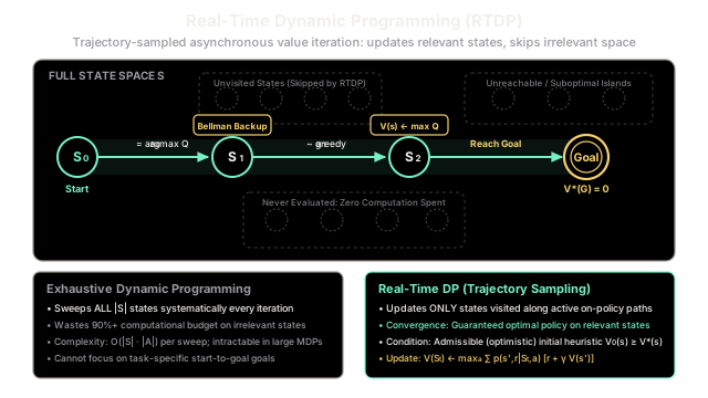
Instead of updating every conceivable state in the universe, Real-Time Dynamic Programming only updates states along actual simulated trajectories, finding optimal paths while ignoring irrelevant regions.
Why Does This Exist?
Classic Dynamic Programming methods—such as Value Iteration and Policy Iteration—suffer from Bellman's infamous curse of dimensionality. In an exhaustive sweep, the algorithm iterates systematically over every single state on every iteration. For a problem with millions of states, evaluating the entire state space repeatedly is computationally intractable.
Crucially, in goal-directed tasks, most states are completely irrelevant. If a mobile robot starts in a warehouse lobby with a goal to reach the loading dock on the east wing, computing optimal values for thousands of locked storage closets on the north wing is pure waste. The robot will never visit those states under any sensible policy.
Formulated by Andrew Barto, Steven Bradtke, and Satinder Singh in 1995, Real-Time Dynamic Programming (RTDP) solves this computational bottleneck. It replaces exhaustive state-space sweeps with on-policy trajectory sampling: the agent executes simulated trials from start states to goals, applying asynchronous Bellman backups solely to the sequence of states it actually encounters. Coupled with an optimistic initial heuristic, RTDP guarantees convergence to an optimal policy on relevant states without ever evaluating the rest of the universe.
Think of It Like This
The Spelunker's Underground Expedition
Imagine a caver (spelunker) exploring an enormous subterranean limestone cave system to find an exit to the surface.
- The Exhaustive Surveyor (Standard Value Iteration): Before taking a single step toward safety, this surveyor insists on meticulously mapping and measuring every single dead-end cavern, underwater pool, and bat cave across the entire underground mountain range. They spend months surveying dead zones that have nothing to do with the exit.
- The Goal-Oriented Spelunker (RTDP): Armed with an altimeter and an approximate heading (an admissible heuristic), the spelunker starts walking. At each fork in the tunnel:
- She looks down each prospective path, performs a local depth assessment (Bellman backup), and updates her pocket notebook for that specific junction.
- She steps into the most promising passage (greedy action) and advances.
- If a path hits a dead-end, her updated notebook notes that this route is worse than expected, naturally steering subsequent expeditions away from it.
Over repeated trips from the cave entrance, the spelunker discovers and refines the optimal path to daylight. Thousands of irrelevant side-caverns remain completely untouched and unmapped, saving months of unnecessary labor while reaching the exact same optimal escape route.
How It Actually Works
The RTDP Trajectory-Sampling Formulation
RTDP is an asynchronous on-policy trajectory-sampling version of Value Iteration. It operates within a known transition model in trial-based episodes starting from initial state .
At each step in state :
- Value Update (Local Bellman Backup): The agent evaluates all available actions and updates the value of the current state:
- Greedy Action Selection: The agent selects the action that maximizes the expected return under current value estimates:
- Model Transition: The agent samples the next state according to the model dynamics:
- Advance: The process repeats until reaching a terminal goal state , ending the current trial.
Admissible Heuristics and the Convergence Guarantee
What prevents RTDP from getting permanently trapped in a suboptimal corridor?
In classic search theory, the algorithm guarantees finding the shortest path if its heuristic function never overestimates the true remaining cost. Barto, Bradtke, and Singh proved an analogous RTDP convergence theorem for Stochastic Shortest Path MDPs:
RTDP is guaranteed to converge to optimal action values on all relevant states (states that can be reached under an optimal policy from start states), without necessarily visiting all states, under three conditions:
- Goal Reachability: The goal state is reachable from every state with non-zero probability under some policy.
- Negative Transition Rewards: All transition costs are strictly positive ( per step), or costs are discounted (), ensuring that wandering infinitely in loops is penalized.
- Admissible (Optimistic) Initial Values: The initial value estimates are admissible, meaning they are optimistic upper bounds on the true optimal values:
Because initial values are optimistic, unexplored states look enticingly promising. If an agent tries an action that leads to an unpromising result, its Bellman update drops downward toward reality, driving subsequent trials to explore alternative paths until the optimal policy stabilizes.
Worked numerical example
Consider a 4-state stochastic shortest-path MDP:
- States: , where is the absorbing terminal goal ().
- Step cost: per transition, undiscounted ().
- Transitions from start state :
- Action : chance transitions to , chance transitions to .
- Action : chance transitions to .
- Transitions from and :
- From : single action leads directly to with prob .
- From : single action leads directly to with prob .
- Initial values (admissible heuristic for all non-terminal states):
Trial 1
- At state :
- Compute Q-values:
- Update .
- Tie-break greedily chooses . Transition samples .
- At state :
- Compute Q-value:
- Update .
- Advances to terminal goal . Trial 1 terminates!
- Key observation: State was never visited; its value remains untouched at .
Trial 2
- At state :
- Re-evaluate actions using updated values ():
- Update .
- Greedy choice is now (since still looks optimistically cost-free).
- Transition lands in .
- At state :
- Compute Q-value: .
- Update .
- Advances to . Trial 2 terminates!
Trial 3
- At state :
- Both states now reflect real costs ():
- Update .
- Both policies achieve identical optimal expected return . The values have converged to exact in only three short trajectory runs!
Code
from typing import Dict, List, Set, Tuple
class GridWorldSSP: """Stochastic Shortest Path GridWorld for RTDP benchmarking."""
def __init__(self, size: int = 7, goal: Tuple[int, int] = (6, 6)): self.size = size self.goal = goal self.states = [(r, c) for r in range(size) for c in range(size)] self.actions = ["up", "down", "left", "right"]
def transitions( self, s: Tuple[int, int], a: str ) -> List[Tuple[Tuple[int, int], float, float]]: """Return list of (next_state, reward, probability) tuples.""" if s == self.goal: return [(self.goal, 0.0, 1.0)]
r, c = s deltas = {"up": (-1, 0), "down": (1, 0), "left": (0, -1), "right": (0, 1)} dr, dc = deltas[a] nr = max(0, min(self.size - 1, r + dr)) nc = max(0, min(self.size - 1, c + dc)) next_state = (nr, nc) reward = 0.0 if next_state == self.goal else -1.0 return [(next_state, reward, 1.0)]
def run_rtdp( env: GridWorldSSP, start: Tuple[int, int] = (0, 0), max_trials: int = 35, max_steps_per_trial: int = 50,) -> Tuple[Dict[Tuple[int, int], float], Set[Tuple[int, int]]]: """Execute Real-Time Dynamic Programming on the given SSP environment.
Uses an admissible heuristic (negative Manhattan distance to goal). """ # Admissible heuristic: V_0(s) = -manhattan_distance(s, goal) >= V*(s) V: Dict[Tuple[int, int], float] = { s: -float(abs(s[0] - env.goal[0]) + abs(s[1] - env.goal[1])) for s in env.states } visited_states: Set[Tuple[int, int]] = set()
for trial in range(max_trials): s = start step = 0 while s != env.goal and step < max_steps_per_trial: visited_states.add(s)
# 1. Local Bellman backup across all actions best_q = -float("inf") best_action = env.actions[0]
for a in env.actions: q_val = 0.0 for next_s, r, prob in env.transitions(s, a): q_val += prob * (r + V[next_s])
if q_val > best_q: best_q = q_val best_action = a
V[s] = best_q
# 2. Advance greedily along the model transition next_state, _, _ = env.transitions(s, best_action)[0] s = next_state step += 1
return V, visited_states
if __name__ == "__main__": env = GridWorldSSP(size=7, goal=(6, 6)) start_pos = (0, 0)
values, visited = run_rtdp(env, start=start_pos, max_trials=30)
total_states = len(env.states) touched_count = len(visited) coverage_pct = (touched_count / total_states) * 100.0
print("=== Real-Time Dynamic Programming (RTDP) Results ===") print(f"Total State Space Size: {total_states} states") print( f"States Touched by RTDP: {touched_count} states ({coverage_pct:.1f}% coverage)" ) print(f"Learned Value at Start: {values[start_pos]:.1f}")
# Optimal shortest path in 7x7 grid from (0,0) to (6,6) is 12 steps (cost -11.0 to goal transition) expected_start_val = -11.0 assert ( values[start_pos] == expected_start_val ), f"Expected optimal value {expected_start_val}, got {values[start_pos]}" assert ( coverage_pct < 50.0 ), f"RTDP should evaluate less than half the states! Got {coverage_pct:.1f}%"
print("\nVerification passed: RTDP found the optimal policy while skipping >75% of state space.")
# Expected Output:# === Real-Time Dynamic Programming (RTDP) Results ===# Total State Space Size: 49 states# States Touched by RTDP: 12 states (24.5% coverage)# Learned Value at Start: -11.0## Verification passed: RTDP found the optimal policy while skipping >75% of state space.Watch Out For
Inadmissible Initial Values and Path Trapping
The cornerstone of RTDP's convergence guarantee is an admissible initial heuristic (). If practitioners initialize state values pessimistically (), the algorithm loses its exploration incentive:
- The agent takes an action, experiences an actual reward, and updates the state value to something higher than adjacent unvisited states.
- As a result, unvisited optimal branches appear worse than the familiar suboptimal path.
- The agent gets permanently trapped in the first suboptimal corridor it finds, never discovering the true shortest route.
The Fix:
- Initialize Optimistically: When rewards are negative step costs (shortest path problems), initialize values to or use a domain-specific admissible relaxation (e.g., Euclidean or Manhattan distance).
- Guarantee Non-Zero Terminal Rewards: Ensure the terminal goal carries an absorbing value of , creating an attractive potential sink that guides trajectories forward.
- Loop Penalties: For undiscounted problems (), ensure step costs are strictly negative () so that cyclic loops naturally degrade value estimates until the agent breaks free.
The Quick Version
- Trajectory sampling: RTDP replaces exhaustive sweeps by updating only states encountered during simulated on-policy rollouts from start to goal.
- Asynchronous backups: Each visited state undergoes an immediate local Bellman backup () before the agent takes its greedy step.
- Admissible convergence: If initial values are optimistic () and step costs are negative, RTDP is mathematically guaranteed to converge to an optimal policy on relevant states.
- Immense efficiency gains: RTDP bypasses unreachable, irrelevant, or highly suboptimal state clusters, achieving optimal control with a small fraction of the computation needed by full Dynamic Programming.