RL Squared (Fast RL via Slow RL)

RL squared trains one recurrent policy slowly across many tasks so that, on a new task, it adapts fast inside its own memory with no weight updates. The hidden state itself becomes the learning algorithm.

RL squared trains a recurrent policy with a slow outer loop so its hidden state carries Trial 1 evidence across the trial boundary and turns Trial 2 nearly greedy, with no weight update at test time.

Why Does This Exist?

Standard RL starts over on every new task. Teach a robot one maze goal and it needs millions of steps; move the goal across the room and training restarts from zero. That is fine for one fixed job and painful for a family of related jobs.

Meta-reinforcement learning changes the objective: train across a distribution of tasks $p(\mathcal{T})$ so a new task $\mathcal{T}_{new}$ takes only a trial or two. MAML in RL answers with gradients: learn an initialization $\theta$ that adapts in one gradient step at test time. That works, and it still pays for a gradient update plus fresh rollouts whenever it meets something new.

RL squared, written RL2 and introduced by Duan et al. in 2016 alongside closely related work by Wang et al., asks a sharper question: what if adaptation lived in memory instead of gradients? Train one recurrent policy slowly with ordinary RL. At test time freeze every weight and let the hidden state do the fast learning as it watches actions, rewards, and done flags stream past. No optimizer runs during deployment. The policy just remembers.

This page covers that memory-as-algorithm trick: the trial-as-sequence setup, the input format that makes it work, and a two-trial bandit trace you can check by hand. For the parent framing read meta-reinforcement learning first. For the memory cell itself see recurrent networks in RL. For the gradient-based sibling, compare MAML in RL.

Think of It Like This

The relief cook with one sticky note

A relief cook covers shifts at many small cafes. Cooking school was the slow loop: months of practice across kitchens that taught knife grip, heat control, and how to read a ticket rail. No single cafe menu was the point. The point was becoming someone who walks into a strange kitchen and gets fast by lunch.

Each shift runs two rushes. The cook carries one sticky note, the fast loop. First rush: table 4 sends back the soup, table 7 orders extra salt, the grill runs hot. Every observation goes on the note. Between rushes the cook keeps the note. That is the whole trick. Second rush: the same dining room, and the note says salty crowd plus hot grill, so seasoning drops and proteins go on thirty seconds later. Orders land.

Shift ends, note goes in the trash. Next cafe means a blank note, because yesterday's regulars say nothing about today's crowd. And the cook never rewrites cooking school during a shift. School shaped how the note gets used. The note does the day's learning.

Where the analogy stops: the cook chooses what to write in words. A recurrent policy's hidden state $h_t$ is a vector shaped only by gradient descent, and nobody reads it directly. You infer what it kept from how Trial 2 behavior changes, the way you would judge the note by the second rush, not by reading it.

How It Actually Works

The trial-as-sequence trick

Fix notation first. A task $\mathcal{T}_i$ is one MDP drawn from $p(\mathcal{T})$ . The policy has weights $\theta$ and a hidden state $h_t$ , the running memory vector. At step $t$ the policy sees the current observation $o_t$ plus its own recent past: the previous action $a_{t-1}$ , the previous reward $r_{t-1}$ , and a done flag $d_{t-1}$ marking trial ends. Then:

$h_{t+1} = f_{\theta}(h_t, o_t, a_{t-1}, r_{t-1}, d_{t-1})$

$a_t \sim \pi_{\theta}(a_t \mid o_t, h_t)$

Here $f_{\theta}$ is the recurrent update (a GRU in the original paper), $\pi_{\theta}$ is the action head reading memory, $o_t$ is what the agent sees now, and $h_t$ summarizes everything it has seen in this episode so far.

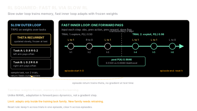
Training, the slow loop, runs a standard policy optimizer (TRPO in the paper) over episodes, where one episode spans several trials on the same sampled task. Trial 1 ends, $d$ flips to mark the boundary, and critically $h$ is kept. Only the episode end clears $h$ back to zero. That kept-across-trials, cleared-across-episodes rule is what turns a plain recurrent policy into a meta-learner: Trial 2 starts already knowing what Trial 1 found.

Test time freezes $\theta$ completely. Adaptation is the forward pass. Trial 1 explores and loads evidence into $h$ . Trial 2 conditions on that loaded $h$ and exploits. Contrast this with MAML, where $\theta$ itself moves by gradient descent on the new task. RL2 moves nothing. It remembers.

The trade is clear. You buy adaptation with zero test-time gradients and pay with a harder training problem plus a narrower comfort zone. The recurrent dynamics must discover something like Bayes-optimal trial behavior from scratch, and they only learn it for the task family they trained on. Outside that family, the memory has no useful prior and Trial 2 looks no smarter than Trial 1. Use RL2 when test tasks come from the same parametric family as training and test-time compute forbids fine-tuning. When tasks shift structurally or you can afford a few gradient steps, prefer an explicit gradient method.

Worked numerical example

Take the paper's simplest demo: a two-armed bandit family with two mirrored tasks. Task A pays $1$ on arm L with probability $0.8$ and on arm R with probability $0.2$ . Task B mirrors it: L pays with $0.2$ , R with $0.8$ . Prior over tasks is $0.5$ each. One episode means two trials of three pulls on the same hidden task. Suppose the hidden task is A.

Trial 1 explores and observes L to $1$ , R to $0$ , L to $1$ . Treat this as the Bayes-optimal reference the trained memory approximates. Likelihood under Task A multiplies per pull:

$P(\text{obs} \mid A) = 0.8 \times 0.8 \times 0.8 = 0.5120$

The middle term is $P(R = 0 \mid A) = 1 - 0.2 = 0.8$ . Under Task B each matching term is $0.2$ :

$P(\text{obs} \mid B) = 0.2 \times 0.2 \times 0.2 = 0.0080$

Bayes with a flat prior gives:

$P(A \mid \text{obs}) = \frac{0.5120}{0.5120 + 0.0080} = 0.9846$

So after three pulls the agent should be $98.5\%$ sure the left arm is good. A trained RL2 policy shows exactly this shape: Trial 1 starts near $P(L) = 0.50$ and Trial 2 sits near $P(L) = 0.98$ , exploiting through $h$ alone. Say Trial 2 pulls L three times and sees $1, 1, 0$ , for $2$ of $3$ .

Expected return makes the gain concrete. An adaptive second trial earns $0.8$ per pull when right about the task and $0.2$ when wrong:

$0.9846 \times 0.8 + 0.0154 \times 0.2 = 0.7908$

That is $2.3723$ over three pulls. A non-adaptive uniform policy earns $0.5$ per pull, or $1.5000$ over three. Memory is worth about $0.87$ extra rewards per trial here. The diagram above draws this same trace: Trial 1 evidence in, posterior $0.9846$ at the boundary, greedy Trial 2 out.

Code

A standalone check of the Trial 1 posterior and the Trial 2 gain. Same numbers as the worked trace:

1from typing import List, Tuple2
3Pull = Tuple[str, int]4
5
6def likelihood(pulls: List[Pull], good_arm: str, p_good: float = 0.8, p_bad: float = 0.2) -> float:7    """Likelihood of pull outcomes if `good_arm` is the high-pay arm."""8    like = 1.09    for arm, reward in pulls:10        p_one = p_good if arm == good_arm else p_bad11        like *= p_one if reward == 1 else (1.0 - p_one)12    return like13
14
15def trial_posterior(pulls: List[Pull]) -> Tuple[float, float, float]:16    """Return (likelihood under A, likelihood under B, posterior of A)."""17    like_a = likelihood(pulls, good_arm="L")18    like_b = likelihood(pulls, good_arm="R")19    return like_a, like_b, like_a / (like_a + like_b)20
21
22if __name__ == "__main__":23    trial1: List[Pull] = [("L", 1), ("R", 0), ("L", 1)]24    like_a, like_b, post_a = trial_posterior(trial1)25    print(f"like_a={like_a:.4f} like_b={like_b:.4f} post_a={post_a:.4f}")26    adaptive = post_a * 0.8 + (1.0 - post_a) * 0.227    print(f"adaptive per pull={adaptive:.4f} x3={adaptive * 3:.4f} uniform x3=1.5000")

1# -> expected output:2like_a=0.5120 like_b=0.0080 post_a=0.98463adaptive per pull=0.7908 x3=2.3723 uniform x3=1.5000

Watch Out For

Clearing memory at the trial boundary erases the lesson

The symptom: Trial 2 performs exactly like Trial 1, and the adaptation gap (Trial 2 return minus Trial 1 return) sits near zero on held-out tasks even though training return looks healthy. The policy explores forever and never exploits.

The usual cause is a reset in the wrong place. Somewhere the rollout code zeroes $h$ whenever $d$ fires, so the trial boundary wipes the evidence Trial 1 just collected. The mirror bug also happens: $h$ is never cleared at the true episode end, so a new task starts with the old task's summary loaded and Trial 1 acts on ghosts.

The fix is mechanical. Keep $h$ across trials inside one episode and clear it only at episode ends. Feed two separate flags if your framework collapses them: one for trial-done (keep memory) and one for episode-done (clear memory). In vectorized rollouts mask per environment, because environments in one batch end episodes on different steps.

Meta-overfitting to a narrow task family

The symptom: training tasks show a fat Trial 2 lift while held-out tasks from a slightly wider range show none. The hidden state memorized which training task it was in rather than learning how to identify tasks. Widening the network changes nothing.

The cause is a task distribution too small to force identification. With two fixed bandit biases the policy can memorize arm identities; with five fixed mazes it can memorize layouts. The outer loop then rewards recognition, not adaptation.

The fix starts with measurement: report the adaptation gap on held-out tasks sampled from a wider range than training, not just training return. Then widen the distribution (randomize payoffs, goal positions, friction), hold out a slice permanently, and stop when the held-out gap stalls. If the gap will not open, the family may need more trials per episode before the memory has enough evidence to matter.

The Quick Version

RL squared trains one recurrent policy slowly across a task family so its hidden state adapts fast at test time with every weight frozen.
Each step feeds the previous action, previous reward, and done flag alongside the observation, and memory persists across the trial boundary inside one episode.
On the two-trial bandit trace, Trial 1 pulls L to 1, R to 0, L to 1 reach posterior $0.9846$ for the left-good task, and Trial 2 turns nearly greedy at $P(L) = 0.98$ .
That memory is worth about $0.87$ extra rewards over three pulls: $2.3723$ expected against $1.5000$ for a non-adaptive policy.
It fails when memory is cleared at trial ends, when stale memory leaks across episodes, and when the task family is too narrow to force real identification.