Semi-Gradient SARSA in RL

Semi-gradient SARSA extends on-policy temporal-difference control to continuous state spaces by approximating action-values with parameterized function approximators. By updating weights using sampled (S, A, R, S', A') transitions, agents learn optimal policies while generalizing across continuous dimensions.

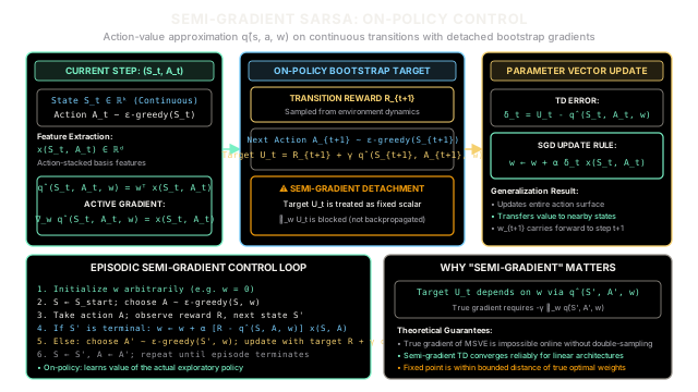
Semi-gradient SARSA updates parameterized action-values on continuous transitions with detached bootstrap gradients.

Why Does This Exist?

In discrete tabular reinforcement learning, SARSA evaluates and improves policies by maintaining a separate table cell $Q(s, a)$ for every state-action pair. However, real-world control domains—such as balancing a pole on a cart, driving a car up a mountain, or controlling a multi-jointed robotic manipulator—operate in continuous state spaces.

In continuous domains, tabular methods collapse completely:

Infinite State Cardinality: Continuous variables (like velocity $\dot{\theta} \in \mathbb{R}$ or position $x \in \mathbb{R}$ ) mean the state space $\mathcal{S}$ is uncountably infinite. A lookup table cannot even be allocated in memory.
Control Demands Action-Values: While state-value methods like semi-gradient TD(0) can estimate $V(s)$ in continuous spaces, state values alone are insufficient for model-free control. Without an environmental transition model $p(s', r \mid s, a)$ , an agent in state $s$ cannot determine which action $a$ leads to the highest-value successor states. The agent must evaluate action-values $q(s, a)$ .

Semi-Gradient SARSA solves the continuous control challenge by extending function approximation directly to action-values:

$\hat{q}(s, a, \mathbf{w}) \approx q_\pi(s, a)$

where $\mathbf{w} \in \mathbb{R}^d$ is a shared parameter vector. By tracking sequential on-policy transitions $(S_t, A_t, R_{t+1}, S_{t+1}, A_{t+1})$ , the algorithm updates its action-value surface online, enabling generalized policy evaluation and $\varepsilon$ -greedy policy improvement across continuous state landscapes.

Think of It Like This

A Racecar Driver Tuning Cornering Technique on an Unfamiliar Track

Imagine an expert racecar driver learning how to navigate an unfamiliar racecourse with a high-performance vehicle:

The Continuous State Space: At any instant mid-corner, the car’s state is defined by continuous physical telemetry: current vehicle speed (e.g., 84.3 mph), lateral g-force, steering angle, and distance to the apex. The driver does not maintain an exhaustive spreadsheet of every possible decimal speed and steering angle.
Action-Value Evaluation ( $q(s, a)$ ): The driver considers distinct tactical inputs: tapping the brakes ( $A_1$ ), feathering the throttle ( $A_2$ ), or holding steady ( $A_3$ ). The driver's mental model predicts the quality of taking throttle action $A_2$ given current telemetry $S$ .
The On-Policy SARSA Transition:
1. Entering the turn at state $S_t$ , the driver chooses action $A_t$ (feather throttle).
2. The car reacts: tires grip, generating immediate reward $R_{t+1}$ (forward velocity without sliding), carrying the car to new telemetry state $S_{t+1}$ .
3. Looking ahead to the next section of asphalt, the driver selects their next intended maneuver $A_{t+1}$ (shift to full throttle for corner exit).
4. The driver updates the value of their initial feather-throttle decision based on the immediate grip ( $R_{t+1}$ ) combined with the anticipated exit speed of the actual next maneuver ( $\gamma \hat{q}(S_{t+1}, A_{t+1})$ ).
The Semi-Gradient Aspect: The driver treats the projected exit speed as a fixed benchmark target during this adjustment. They do not attempt to differentiate the entire mathematical vehicle physics model backward through time.

Where the analogy breaks down: A human driver’s mental model relies on biological neural networks and kinesthetic intuition. In linear Semi-Gradient SARSA, the action-value function is parameterized by an explicit linear feature stack $\mathbf{w}^T \mathbf{x}(s, a)$ optimized via stochastic gradient descent over an episodic Markov decision process.

How It Actually Works

Parameterized Action-Values and Episodic Semi-Gradient Control

Semi-gradient SARSA combines function approximation with the on-policy temporal-difference control loop.

1. Action-Value Function Approximation

The action-value function is approximated by a parameterized function:

$\hat{q}(s, a, \mathbf{w}) \approx q_\pi(s, a)$

In the classical linear case, the approximation is the inner product of parameter vector $\mathbf{w} \in \mathbb{R}^d$ and a joint state-action feature vector $\mathbf{x}(s, a) \in \mathbb{R}^d$ :

$\hat{q}(s, a, \mathbf{w}) \doteq \mathbf{w}^T \mathbf{x}(s, a) = \sum_{i=1}^d w_i x_i(s, a)$

2. Constructing State-Action Features via Action-Stacking

For discrete actions $\mathcal{A} = \{a_1, a_2, \dots, a_m\}$ and continuous state features $\mathbf{x}(s) \in \mathbb{R}^k$ , the canonical representation uses action-stacking (block coding). The global feature vector has dimension $d = k \times m$ :

$\mathbf{x}(s, a_1) = \begin{bmatrix} \mathbf{x}(s) \\ \mathbf{0} \\ \vdots \\ \mathbf{0} \end{bmatrix}, \quad \mathbf{x}(s, a_2) = \begin{bmatrix} \mathbf{0} \\ \mathbf{x}(s) \\ \vdots \\ \mathbf{0} \end{bmatrix}, \quad \dots, \quad \mathbf{x}(s, a_m) = \begin{bmatrix} \mathbf{0} \\ \mathbf{0} \\ \vdots \\ \mathbf{x}(s) \end{bmatrix}$

This structure guarantees that each action maintains its own dedicated subspace within the weight vector $\mathbf{w} = [\mathbf{w}_{a_1}^T, \mathbf{w}_{a_2}^T, \dots, \mathbf{w}_{a_m}^T]^T$ , allowing independent action-value surfaces to evolve without destructive cross-action parameter interference.

3. The On-Policy Semi-Gradient SARSA Update

At time step $t$ , the agent visits continuous state $S_t$ , executes action $A_t$ , observes scalar reward $R_{t+1}$ , and transitions to $S_{t+1}$ . It then samples its next action $A_{t+1}$ using its behavior policy (such as $\varepsilon$ -greedy with respect to $\hat{q}(\cdot, \cdot, \mathbf{w}_t)$ ).

The one-step on-policy SARSA target is:

$U_t \doteq R_{t+1} + \gamma \hat{q}(S_{t+1}, A_{t+1}, \mathbf{w}_t)$

where $\gamma \in [0, 1]$ is the discount factor. If $S_{t+1}$ is a terminal state, the target reduces strictly to $U_t \doteq R_{t+1}$ .

The semi-gradient SGD update rule shifts parameters in the direction of the error gradient:

$\mathbf{w}_{t+1} = \mathbf{w}_t + \alpha \left[ U_t - \hat{q}(S_t, A_t, \mathbf{w}_t) \right] \nabla_{\mathbf{w}} \hat{q}(S_t, A_t, \mathbf{w}_t)$

For linear models, $\nabla_{\mathbf{w}} \hat{q}(S_t, A_t, \mathbf{w}_t) = \mathbf{x}(S_t, A_t)$ , yielding:

$\mathbf{w}_{t+1} = \mathbf{w}_t + \alpha \left[ R_{t+1} + \gamma \hat{q}(S_{t+1}, A_{t+1}, \mathbf{w}_t) - \hat{q}(S_t, A_t, \mathbf{w}_t) \right] \mathbf{x}(S_t, A_t)$

where $\alpha > 0$ is the learning rate.

Why is it called "Semi-Gradient"?

The update is a semi-gradient because the target $U_t = R_{t+1} + \gamma \hat{q}(S_{t+1}, A_{t+1}, \mathbf{w})$ depends on $\mathbf{w}$ . A true gradient of the squared Bellman error $\frac{1}{2}[U_t(\mathbf{w}) - \hat{q}(S_t, A_t, \mathbf{w})]^2$ would include an additional term $-\gamma \nabla_{\mathbf{w}} \hat{q}(S_{t+1}, A_{t+1}, \mathbf{w})$ . Semi-gradient methods intentionally omit this term, treating the target as an exogenous scalar. In linear function approximation, semi-gradient SARSA is provably stable and converges to a bounded region near the optimal TD fixed point.

4. The Complete Episodic Control Loop

1Algorithm: Episodic Semi-Gradient SARSA for Estimating q̂ ≈ q*2───────────────────────────────────────────────────────────────────3Input: a parameterized function q̂(s, a, w) with differentiable weights w4Parameters: step size α > 0, exploration rate ε > 0, discount γ ∈ [0, 1]5Initialize: weight vector w arbitrarily (e.g., w = 0)6
7Loop for each episode:8  S ← initial continuous state9  Choose A ~ ε-greedy based on q̂(S, ·, w)10  Loop for each step of episode:11    Take action A, observe reward R and next state S'12    If S' is terminal:13      w ← w + α [R - q̂(S, A, w)] ∇_w q̂(S, A, w)14      Break (end episode)15    Choose A' ~ ε-greedy based on q̂(S', ·, w)16    w ← w + α [R + γ q̂(S', A', w) - q̂(S, A, w)] ∇_w q̂(S, A, w)17    S ← S', A ← A'

Worked numerical example

Consider a 2-feature linear representation for an action on a single transition step $(S_t, A_t) \xrightarrow{R_{t+1}} (S_{t+1}, A_{t+1})$ .

System Setup

Discount factor: $\gamma = 0.9$
Learning rate: $\alpha = 0.2$
Current parameter weights: $\mathbf{w}_t = [1.0, 0.5]^T$
Active state-action feature vector: $\mathbf{x}(S_t, A_t) = [1.0, 2.0]^T$
Environmental reward observed: $R_{t+1} = +2.0$
Next state-action feature vector: $\mathbf{x}(S_{t+1}, A_{t+1}) = [0.5, 1.0]^T$

Step 1: Compute Current Action-Value Prediction

$\hat{q}(S_t, A_t, \mathbf{w}_t) = \mathbf{w}_t^T \mathbf{x}(S_t, A_t) = (1.0 \times 1.0) + (0.5 \times 2.0) = 1.0 + 1.0 = 2.0000$

Step 2: Compute Next-Action Value Prediction

$\hat{q}(S_{t+1}, A_{t+1}, \mathbf{w}_t) = \mathbf{w}_t^T \mathbf{x}(S_{t+1}, A_{t+1}) = (1.0 \times 0.5) + (0.5 \times 1.0) = 0.5 + 0.5 = 1.0000$

Step 3: Compute On-Policy SARSA Target

$U_t = R_{t+1} + \gamma \hat{q}(S_{t+1}, A_{t+1}, \mathbf{w}_t) = 2.0 + (0.9 \times 1.0000) = 2.0 + 0.9000 = 2.9000$

Step 4: Compute Semi-Gradient TD Error

$\delta_t = U_t - \hat{q}(S_t, A_t, \mathbf{w}_t) = 2.9000 - 2.0000 = +0.9000$

Step 5: Update the Parameter Weight Vector

For a linear model, the gradient is the feature vector itself: $\nabla_{\mathbf{w}} \hat{q}(S_t, A_t, \mathbf{w}_t) = [1.0, 2.0]^T$ .

$\mathbf{w}_{t+1} = \mathbf{w}_t + \alpha \delta_t \mathbf{x}(S_t, A_t) = \begin{bmatrix} 1.0 \\ 0.5 \end{bmatrix} + 0.2 \times 0.9 \times \begin{bmatrix} 1.0 \\ 2.0 \end{bmatrix} = \begin{bmatrix} 1.0 \\ 0.5 \end{bmatrix} + 0.18 \times \begin{bmatrix} 1.0 \\ 2.0 \end{bmatrix} = \begin{bmatrix} 1.0 + 0.18 \\ 0.5 + 0.36 \end{bmatrix} = \begin{bmatrix} 1.1800 \\ 0.8600 \end{bmatrix}$

Step 6: Verify Action-Value Shift

Re-evaluating $(S_t, A_t)$ under the updated weights $\mathbf{w}_{t+1} = [1.18, 0.86]^T$ :

$\hat{q}(S_t, A_t, \mathbf{w}_{t+1}) = (1.18 \times 1.0) + (0.86 \times 2.0) = 1.18 + 1.72 = 2.9000$

The action-value adjusted from $2.0000$ to exactly match the target $2.9000$ , and the updated weights carry forward to guide subsequent decisions across the continuous environment.

Code

Below is a self-contained Python script implementing Linear Semi-Gradient SARSA with action-stacking feature representation, $\varepsilon$ -greedy exploration, and assertions validating both single-step mechanics and continuous navigation convergence:

1import math2import random3from typing import Callable, List, Tuple4
5
6class LinearSemiGradientSARSA:7    """Episodic semi-gradient SARSA control with linear function approximation."""8
9    def __init__(10        self,11        num_features: int,12        actions: List[int],13        alpha: float = 0.2,14        gamma: float = 0.9,15        epsilon: float = 0.1,16    ) -> None:17        self.num_features = num_features18        self.actions = actions19        self.alpha = alpha20        self.gamma = gamma21        self.epsilon = epsilon22        self.weights: List[float] = [0.0] * num_features23
24    def q_value(self, feature_vector: List[float]) -> float:25        """Compute q_hat(s, a, w) = w^T x(s, a)."""26        return sum(w * x for w, x in zip(self.weights, feature_vector))27
28    def select_action(29        self,30        features_for_action: Callable[[int], List[float]],31        explore: bool = True,32    ) -> Tuple[int, List[float]]:33        """Select action using epsilon-greedy policy over candidate feature vectors."""34        if explore and random.random() < self.epsilon:35            chosen_action = random.choice(self.actions)36            return chosen_action, features_for_action(chosen_action)37
38        best_a = self.actions[0]39        best_features = features_for_action(best_a)40        best_q = self.q_value(best_features)41
42        for a in self.actions[1:]:43            features = features_for_action(a)44            q = self.q_value(features)45            if q > best_q:46                best_q = q47                best_a = a48                best_features = features49
50        return best_a, best_features51
52    def update(53        self,54        curr_features: List[float],55        reward: float,56        next_features: List[float],57        is_terminal: bool,58    ) -> Tuple[float, float]:59        """Perform a single 1-step semi-gradient SARSA parameter update."""60        q_curr = self.q_value(curr_features)61        q_next = 0.0 if is_terminal else self.q_value(next_features)62
63        # On-policy TD target: U = R + gamma * q_hat(S', A', w)64        target = reward + self.gamma * q_next65        delta = target - q_curr66
67        # Gradient of linear q_hat w.r.t w is curr_features68        for i in range(len(self.weights)):69            self.weights[i] += self.alpha * delta * curr_features[i]70
71        return delta, target72
73
74def run_sarsa_demonstration() -> None:75    # Part 1: Worked Numerical Walkthrough Verification76    agent = LinearSemiGradientSARSA(num_features=2, actions=[0, 1], alpha=0.2, gamma=0.9)77    agent.weights = [1.0, 0.5]78
79    x_curr = [1.0, 2.0]80    x_next = [0.5, 1.0]81    reward = 2.082
83    q_curr = agent.q_value(x_curr)84    q_next = agent.q_value(x_next)85    print("--- Single-Step Worked Numerical Walkthrough ---")86    print(f"Initial q(S_t, A_t):     {q_curr:.4f}")87    print(f"Next q(S_t+1, A_t+1):   {q_next:.4f}")88
89    delta, target = agent.update(x_curr, reward, x_next, is_terminal=False)90    print(f"SARSA Target:           {target:.4f}")91    print(f"TD Error delta:         {delta:.4f}")92    print(f"Updated weights w:      [{agent.weights[0]:.4f}, {agent.weights[1]:.4f}]")93
94    assert abs(q_curr - 2.0) < 1e-695    assert abs(q_next - 1.0) < 1e-696    assert abs(target - 2.9) < 1e-697    assert abs(delta - 0.9) < 1e-698    assert abs(agent.weights[0] - 1.18) < 1e-699    assert abs(agent.weights[1] - 0.86) < 1e-6100
101    # Part 2: Continuous 1D Navigation Control Task102    # State s in [0.0, 10.0]. Action 0: move left (-1.0), Action 1: move right (+1.0)103    # Terminal Goal: reach s >= 9.5 (Reward = +10.0, step cost = -0.1)104    # Action-stacking feature representation: 2 base features * 2 actions = 4 features105    def make_stacked_features(state: float, action: int) -> List[float]:106        base_features = [state / 10.0, 1.0]107        if action == 0:108            return base_features + [0.0, 0.0]109        else:110            return [0.0, 0.0] + base_features111
112    control_agent = LinearSemiGradientSARSA(113        num_features=4, actions=[0, 1], alpha=0.1, gamma=0.95, epsilon=0.1114    )115
116    random.seed(42)117    # Train across 100 episodes118    for ep in range(100):119        s = random.uniform(1.0, 7.0)120        a, feats = control_agent.select_action(lambda act: make_stacked_features(s, act))121        done = False122        steps = 0123        while not done and steps < 40:124            steps += 1125            s_next = max(0.0, min(10.0, s + (1.0 if a == 1 else -1.0)))126            done = s_next >= 9.5127            r = 10.0 if done else -0.1128
129            if done:130                control_agent.update(feats, r, [], is_terminal=True)131            else:132                a_next, feats_next = control_agent.select_action(133                    lambda act: make_stacked_features(s_next, act)134                )135                control_agent.update(feats, r, feats_next, is_terminal=False)136                s, a, feats = s_next, a_next, feats_next137
138    # Evaluate learned policy at midpoint s = 5.0139    q_left = control_agent.q_value(make_stacked_features(5.0, 0))140    q_right = control_agent.q_value(make_stacked_features(5.0, 1))141
142    print("\n--- Continuous Navigation Control Results ---")143    print(f"Midpoint s=5.0 Q(move_left):  {q_left:.4f}")144    print(f"Midpoint s=5.0 Q(move_right): {q_right:.4f}")145    print(f"Learned weights w:            {[round(w, 4) for w in control_agent.weights]}")146
147    # Moving right toward goal should have substantially higher value than moving left148    assert q_right > q_left + 1.0149
150
151if __name__ == "__main__":152    run_sarsa_demonstration()153
154# -> Expected output:155# -> --- Single-Step Worked Numerical Walkthrough ---156# -> Initial q(S_t, A_t):     2.0000157# -> Next q(S_t+1, A_t+1):   1.0000158# -> SARSA Target:           2.9000159# -> TD Error delta:         0.9000160# -> Updated weights w:      [1.1800, 0.8600]161# -> 162# -> --- Continuous Navigation Control Results ---163# -> Midpoint s=5.0 Q(move_left):  6.1970164# -> Midpoint s=5.0 Q(move_right): 7.7725165# -> Learned weights w:            [2.8601, 4.767, 5.976, 4.7845]

Watch Out For

Policy Chattering and the Danger of Off-Policy Max Backups

Two prominent stability traps threaten control algorithms when transitioning from tabular to function approximation:

1. Policy Chattering at Decision Boundaries: In tabular control, once $Q(s, a_1) > Q(s, a_2)$ , the greedy policy remains solidly locked on $a_1$ . In function approximation, updating the value of an action in a neighboring state alters weights across the shared feature space. Near decision boundaries, small parameter adjustments cause the dominant action to flip-flop rapidly between $a_1$ and $a_2$ on alternate steps—a pathology called policy chattering. The Fix: Use conservative learning rates ( $\alpha$ ), decayed exploration schedules, and smooth feature representations (such as overlapping tile codings or soft action distributions like softmax policies) to prevent erratic boundary oscillations.

2. The Off-Policy Max-Operator Trap (The Deadly Triad): Practitioners frequently attempt to replace SARSA's on-policy target with an off-policy Q-learning target: $U = R + \gamma \max_a \hat{q}(S', a, \mathbf{w})$ . When combined with function approximation and bootstrapping, the $\max$ operator forms the notorious Deadly Triad. Because off-policy distribution mismatch interacts destructively with bootstrapping, linear Q-learning can spiral into unbounded parameter divergence! The Fix: Stick with on-policy Semi-Gradient SARSA for guaranteed linear stability. If off-policy control is mandatory, use target networks to freeze bootstrap parameters or employ Gradient-TD methods that explicitly minimize projected Bellman errors.

The Quick Version

Continuous Action-Value Control: Semi-gradient SARSA scales temporal-difference control to continuous state spaces by parameterizing action-values as $\hat{q}(s, a, \mathbf{w}) \approx q_\pi(s, a)$ .
Action-Stacked Features: Discrete actions are typically handled by stacking state features into disjoint blocks $\mathbf{x}(s, a)$ , allowing independent linear action-value surfaces to evolve without destructive parameter interference.
On-Policy Bootstrapping: Updates evaluate the actual next action $A_{t+1} \sim \pi(\cdot \mid S_{t+1})$ , ensuring that targets remain on-policy and avoiding the divergent instabilities of the Deadly Triad.
Semi-Gradient Detachment: The algorithm ignores the target's mathematical dependency on $\mathbf{w}$ , treating $R_{t+1} + \gamma \hat{q}(S_{t+1}, A_{t+1}, \mathbf{w}_t)$ as a fixed scalar to ensure stable SGD weight updates.