Tabular Solution Methods

Tabular solution methods represent value functions and policies as exact discrete lookup tables, enabling precise updates for small state and action spaces without function approximation.

Tabular reinforcement learning maintains an explicit matrix of state-action values, updating targeted memory cells directly without interference across unvisited states.

Why Does This Exist?

In reinforcement learning, an agent must evaluate how promising states and actions are to form an optimal policy. In the simplest and most mathematically rigorous setting, the state space $\mathcal{S}$ and action space $\mathcal{A}$ are finite and small enough that an agent can store every value explicitly in memory. These approaches are known as tabular solution methods.

When an agent uses parameterized function approximators like deep neural networks, updating the value estimate of one state modifies the network weights, which unintentionally alters the predicted values of other, unvisited states. This phenomenon—known as generalization or cross-state interference—can destabilize learning, induce catastrophic forgetting, or cause divergence when combined with bootstrapping and off-policy sampling (the Deadly Triad).

Tabular methods exist because they eliminate cross-state interference entirely. Modifying the entry for $(s, a)$ alters only that specific memory cell, leaving all other state-action estimates bit-for-bit unchanged. This total decoupling provides the theoretical proving ground for reinforcement learning: classical convergence proofs for Dynamic Programming, Monte Carlo evaluation, SARSA, and Q-learning rely on tabular representations to guarantee exact convergence to the true optimal value functions $V^*$ and $Q^*$ .

Think of It Like This

The Crossroads Ledger

Imagine a courier traveling between a small network of numbered crossroads. In their satchel, the courier carries a physical paper ledger.

Every page corresponds to a specific crossroad (state $s$ ), and every column on that page corresponds to an outgoing path (action $a$ ). Each cell contains a penciled number: the expected delivery bonus (value estimate) associated with taking that road.

When the courier takes path $a_1$ from crossroad $S_2$ and collects a toll reward, they open to page $S_2$ , erase the number in column $a_1$ , and pencil in an updated estimate. Because they are writing on a physical paper cell, updating page $S_2$ has zero effect on page $S_1$ or page $S_3$ . The records remain cleanly isolated.

The analogy breaks down when the courier must navigate an entire continent with continuous GPS coordinates or millions of intersections. A paper ledger would require an impossible number of pages, and the courier would have to visit every single intersection multiple times from scratch; the notebook cannot automatically infer what a new crossroads looks like based on familiar ones.

How It Actually Works

State-Action Value Arrays and Exact Bellman Backups

In tabular reinforcement learning, the state value function $V$ and the action-value function $Q$ are represented as multidimensional arrays indexed directly by discrete state and action identities:

State-value array: $V \in \mathbb{R}^{|\mathcal{S}|}$ , where entry $V[s]$ stores the expected return starting from state $s \in \mathcal{S}$ .
Action-value matrix: $Q \in \mathbb{R}^{|\mathcal{S}| \times |\mathcal{A}|}$ , where entry $Q[s, a]$ stores the expected return starting from state $s \in \mathcal{S}$ and taking action $a \in \mathcal{A}$ .

Because every state and action corresponds to an exact table coordinate, updates to the value functions operate via direct assignment rather than gradient descent over parameter vectors.

In model-based tabular dynamic programming, the Bellman expectation backup for state values evaluates all possible transition branches:

V(s) \leftarrow \sum_{a \in \mathcal{A}} \pi(a|s) \sum_{s' \in \mathcal{S}} \sum_{r} p(s', r | s, a) \left[ r + \gamma V(s') \right]

where:

$\pi(a|s)$ is the probability of selecting action $a$ in state $s$ under policy $\pi$ .
$p(s', r | s, a)$ is the joint probability of transitioning to state $s'$ with reward $r$ .
$\gamma \in [0, 1)$ is the discount factor for future rewards.

In model-free sample-based settings (such as tabular Q-learning), the agent receives a transition tuple $(s_t, a_t, R_{t+1}, s_{t+1})$ from interaction and computes the Temporal Difference (TD) error:

\delta_t = R_{t+1} + \gamma \max_{a'} Q(s_{t+1}, a') - Q(s_t, a_t)

The Q-table entry is then updated in place:

Q(s_t, a_t) \leftarrow Q(s_t, a_t) + \alpha_t(s_t, a_t) \, \delta_t

where $\alpha_t(s_t, a_t) \in (0, 1]$ is the step-size parameter (learning rate).

Exact Convergence Guarantees

Under tabular representations, the Bellman optimality operator $T^*$ defined by:

(T^* Q)(s, a) = \sum_{s', r} p(s', r | s, a) \left[ r + \gamma \max_{a'} Q(s', a') \right]

is a $\gamma$ -contraction mapping under the maximum norm $\| Q \|_\infty = \max_{s, a} |Q(s, a)|$ :

\| T^* Q_1 - T^* Q_2 \|_\infty \le \gamma \| Q_1 - Q_2 \|_\infty

By Banach's Fixed Point Theorem, repeated application of $T^*$ converges to a unique fixed point $Q^*$ . For stochastic sample updates, tabular Q-learning is guaranteed to converge almost surely to $Q^*$ provided all state-action pairs continue to be visited infinitely often and the step-size schedule satisfies the standard Robbins-Monro conditions:

\sum_{t=1}^\infty \alpha_t(s, a) = \infty \quad \text{and} \quad \sum_{t=1}^\infty \alpha_t^2(s, a) < \infty \quad \forall (s, a) \in \mathcal{S} \times \mathcal{A}

Worked numerical example

Consider a 4-state Markov Decision Process chain:

State space: $\mathcal{S} = \{S_0, S_1, S_2, S_3\}$ , where $S_3$ is an absorbing terminal state.
Action space: $\mathcal{A} = \{a_0 (\text{Left}), a_1 (\text{Right})\}$ .
Hyperparameters: Learning rate $\alpha = 0.50$ , discount factor $\gamma = 0.90$ .

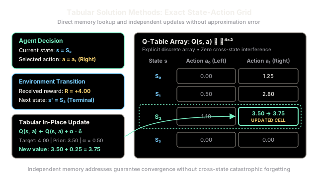
Before the step, the agent's Q-table stores the following estimates:

State	$Q(s, a_0)$ [Left]	$Q(s, a_1)$ [Right]
$S_0$	$0.00$	$1.25$
$S_1$	$0.50$	$2.80$
$S_2$	$1.10$	$3.50$
$S_3$ (terminal)	$0.00$	$0.00$

The agent is currently in state $s = S_2$ and selects action $a = a_1$ (Right). The environment transitions to next state $s' = S_3$ (terminal) and yields an immediate scalar reward $R = +4.00$ .

Current Cell Lookup: Retrieve the active table entry: $Q(S_2, a_1) = 3.50$
Next-State Value Evaluation: Because $S_3$ is a terminal absorbing state, all future expected return is zero: $\max_{a'} Q(S_3, a') = 0.00$
Compute the TD Target: Combine the immediate payoff with the discounted downstream value: $\text{TD Target} = R + \gamma \max_{a'} Q(S_3, a') = 4.00 + 0.90 \times 0.00 = 4.00$
Compute the TD Error ( $\delta$ ): $\delta = \text{TD Target} - Q(S_2, a_1) = 4.00 - 3.50 = +0.50$
In-Place Cell Write: Update table cell $(S_2, a_1)$ using step size $\alpha = 0.50$ : $Q(S_2, a_1) \leftarrow 3.50 + 0.50 \times 0.50 = 3.50 + 0.25 = 3.75$

Notice that $Q(S_2, a_0) = 1.10$ and all values for $S_0, S_1,$ and $S_3$ remain completely unchanged. The update is strictly local.

Code

1from typing import List, Tuple2
3
4class TabularQTable:5    """Explicit 2D lookup table storing discrete state-action values Q(s, a)."""6
7    def __init__(self, num_states: int, num_actions: int, default_value: float = 0.0) -> None:8        self.num_states: int = num_states9        self.num_actions: int = num_actions10        # 2D table representing Q in R^(|S| x |A|) with exact isolated entries11        self.table: List[List[float]] = [12            [default_value for _ in range(num_actions)] for _ in range(num_states)13        ]14
15    def get_value(self, state: int, action: int) -> float:16        """Retrieve the exact action-value stored for pair (state, action)."""17        return self.table[state][action]18
19    def set_value(self, state: int, action: int, value: float) -> None:20        """Directly write an updated return estimate to a single cell."""21        self.table[state][action] = value22
23    def best_action(self, state: int) -> int:24        """Return the greedy action that maximizes the estimated return."""25        action_values = self.table[state]26        best_act = 027        best_val = action_values[0]28        for act in range(1, self.num_actions):29            if action_values[act] > best_val:30                best_val = action_values[act]31                best_act = act32        return best_act33
34    def update(35        self,36        state: int,37        action: int,38        reward: float,39        next_state: int,40        done: bool,41        alpha: float = 0.5,42        gamma: float = 0.9,43    ) -> Tuple[float, float]:44        """Apply an in-place tabular Q-learning update to cell (state, action)."""45        current_q = self.table[state][action]46        next_max = 0.0 if done else max(self.table[next_state])47        td_target = reward + gamma * next_max48        td_error = td_target - current_q49        new_q = current_q + alpha * td_error50        self.table[state][action] = new_q51        return td_error, new_q52
53
54# Initialize a 4-state, 2-action chain environment55q_table = TabularQTable(num_states=4, num_actions=2)56
57# Load existing estimated returns for states S0 through S358q_table.table[0] = [0.00, 1.25]59q_table.table[1] = [0.50, 2.80]60q_table.table[2] = [1.10, 3.50]61q_table.table[3] = [0.00, 0.00]  # Terminal absorbing state62
63print(f"Initial Q(S2, a1): {q_table.get_value(state=2, action=1):.2f}")64
65# Experience transition: S2 -> action a1 -> reward +4.00 -> next state S3 (terminal)66td_err, updated_val = q_table.update(67    state=2, action=1, reward=4.0, next_state=3, done=True, alpha=0.5, gamma=0.968)69
70print(f"TD Error: {td_err:.2f}")71print(f"Updated Q(S2, a1): {updated_val:.2f}")72print(f"Untouched Q(S2, a0): {q_table.get_value(state=2, action=0):.2f}")73# -> Initial Q(S2, a1): 3.5074# -> TD Error: 0.5075# -> Updated Q(S2, a1): 3.7576# -> Untouched Q(S2, a0): 1.10

Watch Out For

The Curse of Dimensionality and State Space Explosion

Attempting to apply tabular solution methods to environments with continuous, high-dimensional, or combinatorial state spaces triggers exponential explosion in memory and sample requirements.

If a robotic arm state is described by $d = 8$ joint angles and velocities, and each continuous variable is discretized into just $k = 20$ bins, the state table requires:

|\mathcal{S}| = k^d = 20^8 = 2.56 \times 10^{10} \text{ distinct states}

Storing this table requires hundreds of gigabytes of RAM. More critically, sample complexity explodes: because tabular methods possess zero inductive bias or generalization between states, learning an accurate value for state $(s_1, s_2, \dots, s_d)$ provides literally zero information about the neighboring state $(s_1 + \epsilon, s_2, \dots, s_d)$ . An agent would need billions of interaction steps just to visit each cell once.

When the state space exceeds tens of thousands of discrete states, stop using tabular lookup tables and transition to function approximation methods such as tile coding, radial basis functions, or deep neural networks (e.g., Deep Q-Networks).

The Quick Version

Tabular solution methods represent value functions $V(s)$ and $Q(s, a)$ as explicit arrays or lookup matrices over discrete state and action spaces.
Updates are strictly localized: writing to cell $(s, a)$ produces zero cross-talk, distortion, or catastrophic forgetting in any other state entry.
Under finite spaces and standard step-size schedules, tabular Dynamic Programming and Temporal Difference methods enjoy absolute mathematical convergence guarantees to optimal policies.
The approach is fundamentally limited by the curse of dimensionality ( $O(|\mathcal{S}| \cdot |\mathcal{A}|)$ ) and cannot generalize knowledge to unseen or continuous states without function approximation.