Advanced Tabular Methods
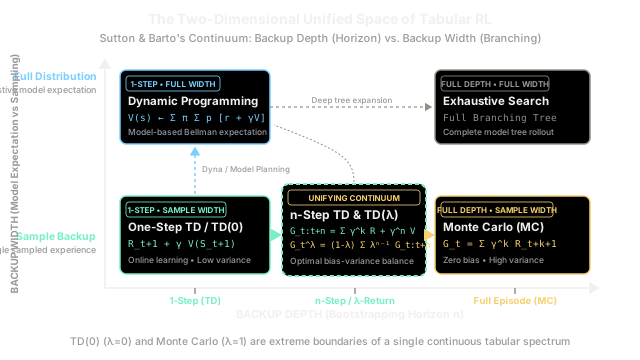
Reinforcement learning algorithms do not exist as isolated methods, but as coordinates across a continuous two-dimensional spectrum defined by backup depth and backup width. By varying the bootstrapping horizon from one step to an entire episode, advanced tabular methods smoothly bridge temporal-difference learning and Monte Carlo methods.
Why Does This Exist?
Introductory reinforcement learning texts often introduce Dynamic Programming, Monte Carlo Methods, and Temporal Difference Learning as three rival, disconnected paradigms. Practitioners are taught to make a binary decision: either assume a known transition model and run dynamic programming sweeps, or sample trial-and-error experience model-free using TD or Monte Carlo.
This siloed perspective breaks down in practice because extreme algorithmic choices carry severe theoretical and practical penalties:
- Pure One-Step TD (TD(0)) bootstraps immediately after a single transition. It updates value estimates online without waiting for an episode to terminate, yielding low sample variance. However, when value tables are initialized arbitrarily or poorly approximated, bootstrapping compounds estimation bias, causing credit assignment for distant terminal rewards to propagate backward agonizingly slowly—one state per episode.
- Pure Monte Carlo waits until an episode terminates to tally the complete empirical return. Because it uses actual observed outcomes rather than value estimates, it is completely unbiased with respect to future bootstrapping errors. Yet its variance is extreme: every random action and stochastic environment transition along an extended trajectory compounds exponentially, demanding vast quantities of data to converge. Furthermore, Monte Carlo cannot learn during an ongoing task or in non-terminating, continuing environments.
Advanced tabular methods exist to unify these seemingly disparate algorithms into a single mathematical continuum. By introducing -step returns and eligibility traces, Richard Sutton and Andrew Barto mapped all tabular learning onto a unified two-dimensional coordinate space defined by backup depth (how many time steps forward an agent looks before bootstrapping) and backup width (whether the update averages across all possible model transitions or follows a single sampled trajectory).
Unification transforms algorithmic selection from an either-or compromise into a continuous hyperparameter tuning problem, allowing agents to strike an optimal balance between bias and variance.
Think of It Like This
The Electromagnetic Spectrum of Vision
For centuries, natural philosophers discovered and named electromagnetic phenomena as though they were completely unrelated forces of nature. Marconi built radio antennas; Roentgen uncovered penetrating X-rays; Herschel measured invisible thermal infrared heat; and human eyes perceived red, green, and violet light. Each phenomenon required distinct sensors, mathematics, and operational hardware.
It was not until James Clerk Maxwell formulated classical electromagnetism that physicists realized radio waves, visible colors, and X-rays are identical physical entities: electromagnetic radiation propagating at the speed of light. They differ only along a single continuous scalar axis: wavelength (or frequency). Visible light is simply a narrow band in the middle of a continuous physical spectrum.
In tabular reinforcement learning, TD(0) and Monte Carlo are the radio waves and gamma rays of credit assignment:
- TD(0) is like high-frequency gamma radiation: hyper-localized, tightly focused on the immediate nanosecond transition, and blind to what happens ten minutes later.
- Monte Carlo is like low-frequency radio waves: massive wavelengths spanning the entire length of the episode from the opening move to the terminal buzzer, capturing broad macro returns while accumulating environmental static.
Advanced tabular methods reveal that TD(0) and Monte Carlo are not different algorithms; they are the extreme left and right ends of the -step spectrum. Intermediate methods like 3-step TD or operate in the visible light spectrum: they look ahead several steps to capture true reward signals while bootstrapping early enough to filter out downstream noise.
Where the analogy stops: Electromagnetic radiation travels across empty space at the speed of light regardless of wavelength. In reinforcement learning, extending the backup depth incurs a real computational and temporal delay: an -step algorithm must buffer transitions and wait real environment steps before it can compute an update to state .
How It Actually Works
The Two-Dimensional Unified Space and the n-Step Continuum
Sutton & Barto organize all tabular reinforcement learning algorithms across two orthogonal dimensions:
Backup Width (Degree of Distributional Expectation) ▲ │ [Dynamic Programming] [Exhaustive Search] │ Full distribution backup Full distribution tree rollout │ Depth = 1 step, Width = Full Depth = ∞, Width = Full │ │ [Dyna / Model-Based Planning] [Monte Carlo Tree Search] │ Intermediate width Branching sampled rollouts │ │ [One-Step TD / TD(0)] ──► [n-Step TD & TD(λ)] ──► [Monte Carlo] │ Single sample backup Bridging continuum Single sample rollout │ Depth = 1 step, Width = 1 Depth = n, Width = 1 Depth = ∞, Width = 1 └─────────────────────────────────────────────────────────────► Backup Depth 1-Step Intermediate n Full Episode (∞)- Backup Depth (Horizontal Axis): Governs how far into the future the agent accumulates true sampled rewards before bootstrapping off the estimated value of the subsequent state.
- Backup Width (Vertical Axis): Governs the branching factor of the backup. A sample backup (model-free) follows the single transition actually sampled by the environment. A full distribution backup (model-based Dynamic Programming) uses transition probabilities to compute the exhaustive mathematical expectation across all potential outcomes.
The n-Step Return Formulation
Let an agent generate a trajectory of states, actions, and rewards:
where:
- is the state visited at time .
- is the action taken at time .
- is the numerical reward received after transition.
- is the discount factor for future rewards.
- is the terminal time step of the episode.
- is the tabular value estimate of state available at time step .
The generalized -step return accumulates discounted rewards and bootstraps using the value estimate of the state reached at step :
If (the horizon extends beyond episode termination), the bootstrapping term vanishes, and the -step return truncates to the complete episodic return:
The tabular value update rule applied at time step (once the required steps of experience have been observed) is:
where is the step-size learning rate parameter.
Notice how the boundaries recover classical algorithms exactly:
- When : , recovering standard one-step TD(0).
- When (or ): , recovering full Monte Carlo.
The Compound -Return and Eligibility Traces Bridge
Rather than selecting a single fixed horizon , advanced tabular methods can average multiple -step returns. The -return combines every possible -step return into a single compound target using a geometric weighting parameterized by :
The weighting terms form a geometric progression that sums to :
- Setting places of the weight on , recovering TD(0).
- Setting places all weight on the terminal Monte Carlo return .
- Setting smoothly interpolates across all horizons simultaneously.
While computing directly (the forward view) requires looking ahead until the end of the episode, the backward view of Eligibility Traces uses short-term memory traces to produce the exact same total weight updates online and incrementally at every time step with complexity per transition:
Worked numerical example
Consider an agent navigating a 4-step trajectory that terminates at state :
Let the discount factor be and the step-size learning rate be .
The initial tabular state-value estimates are:
- (terminal state value is identically zero)
We compute the updated value using different backup depths along the spectrum.
Step 1: Compute n-Step Returns for
-
One-step return (, TD(0)):
-
Two-step return ():
-
Three-step return ():
-
Four-step return (, full Monte Carlo return ):
Step 2: Compute the Compound -Return for
The episode length is . For , we evaluate the geometric weights assigned to each -step return:
- Weight for :
- Weight for :
- Weight for :
- Weight for (terminal remainder):
Check sum of weights:
The compound -return is:
Step 3: Compare Value Updates for
Applying the update rule with and initial :
- TD(0) ():
- Compound -Return ():
- Monte Carlo ():
Notice how the target scales monotonically from up to . Pure TD(0) under-reacts because it relies heavily on the underestimated initial table entry . Pure Monte Carlo captures the large reward directly but is vulnerable to trajectory variance in stochastic domains. The intermediate -return strikes a balanced compromise at .
Code
from typing import Dict, List, Tuple
def compute_n_step_return( rewards: List[float], states: List[int], values: Dict[int, float], gamma: float, start_t: int, n: int,) -> float: """Compute the n-step return G_{t:t+n} for starting step t. Args: rewards: Sequence of observed rewards [R_1, R_2, ..., R_T]. states: Sequence of visited states [S_0, S_1, ..., S_T]. values: Tabular dictionary mapping discrete state ids to value estimates. gamma: Discount factor in [0, 1]. start_t: Origin time step t being evaluated. n: Number of backup steps (horizon window).
Returns: The calculated n-step return G_{t:t+n}. """ horizon = len(rewards) end_t = min(start_t + n, horizon)
# Accumulate discounted rewards over the n-step window discounted_reward_sum = 0.0 for k in range(start_t, end_t): discounted_reward_sum += (gamma ** (k - start_t)) * rewards[k]
# Bootstrap from estimated value of state reached at start_t + n target_idx = start_t + n if target_idx <= horizon: bootstrap_state = states[target_idx] bootstrap_val = (gamma ** n) * values.get(bootstrap_state, 0.0) else: bootstrap_val = 0.0
return discounted_reward_sum + bootstrap_val
def compute_lambda_return( rewards: List[float], states: List[int], values: Dict[int, float], gamma: float, start_t: int, lam: float,) -> Tuple[float, List[Tuple[int, float, float]]]: """Compute the compound lambda-return as a geometric mixture of n-step returns.
Args: rewards: Sequence of observed rewards [R_1, ..., R_T]. states: Sequence of visited states [S_0, ..., S_T]. values: Tabular state-value dictionary. gamma: Discount factor. start_t: Starting time step. lam: Lambda parameter in [0, 1].
Returns: A tuple of (compound_return, list_of_tuples(n, return_n, weight_n)). """ horizon = len(rewards) remaining_steps = horizon - start_t n_step_data: List[Tuple[int, float, float]] = [] compound_return = 0.0
for n in range(1, remaining_steps + 1): g_n = compute_n_step_return(rewards, states, values, gamma, start_t, n) if n < remaining_steps: weight = (1.0 - lam) * (lam ** (n - 1)) else: weight = lam ** (n - 1) # Terminal remainder absorbs residual weight n_step_data.append((n, g_n, weight)) compound_return += weight * g_n
return compound_return, n_step_data
# Trajectory: S0 -> S1 -> S2 -> S3 -> S4 (terminal)trajectory_states = [0, 1, 2, 3, 4]trajectory_rewards = [2.0, 1.0, 4.0, 10.0]state_values = {0: 0.0, 1: 3.0, 2: 5.0, 3: 8.0, 4: 0.0}discount = 0.9alpha = 0.2
print("=== N-Step Returns from State S0 ===")for n in range(1, 5): ret = compute_n_step_return( trajectory_rewards, trajectory_states, state_values, discount, 0, n ) label = "TD(0)" if n == 1 else ("Monte Carlo" if n == 4 else f"{n}-Step") print(f"n={n} ({label:11s}): Return = {ret:6.2f} | Updated V(S0) = {alpha * ret:5.2f}")
lam_val = 0.5lam_ret, details = compute_lambda_return( trajectory_rewards, trajectory_states, state_values, discount, 0, lam_val)
print(f"\n=== Compound Lambda-Return (lambda={lam_val}) ===")for n, g_n, w in details: print(f"n={n}: Return = {g_n:6.2f}, Weight = {w:5.3f}, Component = {w*g_n:5.2f}")print(f"Total G_0^(lambda={lam_val}): {lam_ret:.2f} | Updated V(S0): {alpha * lam_ret:.2f}")
# -> === N-Step Returns from State S0 ===# -> n=1 (TD(0) ): Return = 4.70 | Updated V(S0) = 0.94# -> n=2 (2-Step ): Return = 6.95 | Updated V(S0) = 1.39# -> n=3 (3-Step ): Return = 11.97 | Updated V(S0) = 2.39# -> n=4 (Monte Carlo): Return = 13.43 | Updated V(S0) = 2.69# -> # -> === Compound Lambda-Return (lambda=0.5) ===# -> n=1: Return = 4.70, Weight = 0.500, Component = 2.35# -> n=2: Return = 6.95, Weight = 0.250, Component = 1.74# -> n=3: Return = 11.97, Weight = 0.125, Component = 1.50# -> n=4: Return = 13.43, Weight = 0.125, Component = 1.68# -> Total G_0^(lambda=0.5): 7.26 | Updated V(S0): 1.45Watch Out For
Treating TD, DP, and MC as Isolated Algorithm Silos
Practitioners frequently treat Dynamic Programming, TD(0), and Monte Carlo as mutually exclusive software silos. When an algorithm underperforms on a task, teams often throw out the algorithm class entirely—switching from TD to pure Monte Carlo or vice versa—rather than tuning the continuous dials of the unified space.
Failure Mode and Symptoms:
- Sluggish Credit Assignment under TD(0): In mazes or games where rewards occur only at episode termination, pure TD(0) () propagates reward information backward by exactly one state per completed episode. A 100-step trajectory requires hundreds of episodes before the initial state receives any non-zero gradient, stalling training progress.
- Variance Explosion under Monte Carlo: In environments with stochastic transition dynamics (e.g., wind slippage or random market shocks), pure Monte Carlo () aggregates noise across every step. Trajectory variance compounds multiplicatively, causing value estimates to fluctuate wildly and requiring millions of samples to stabilize.
Concrete Fix: Diagnose where your task lies on the two-dimensional spectrum:
- Along the Width Axis: If a model of transition dynamics is partially known or learnable, use simulated background updates (e.g., the Dyna architecture) to interpolate between single-sample backups and full Bellman expectations.
- Along the Depth Axis: Do not settle for the extremes or . Run a hyperparameter search across or implement eligibility traces () with . An intermediate horizon lets real reward signals travel multiple steps backward immediately while cutting off downstream trajectory noise with a bootstrapped estimate.
The Quick Version
- Tabular reinforcement learning is a continuous two-dimensional design space governed by backup depth (bootstrapping horizon) and backup width (sample versus distribution).
- One-step TD(0) () and full Monte Carlo () are the two extreme boundaries of a single continuous spectrum of -step returns.
- Increasing backup depth decreases inductive bias from inaccurate bootstrap values but increases sample variance across stochastic transitions.
- The compound -return and eligibility traces () smoothly combine all -step horizons simultaneously, enabling online credit assignment with an optimal bias-variance balance.