Tree-Backup Algorithm
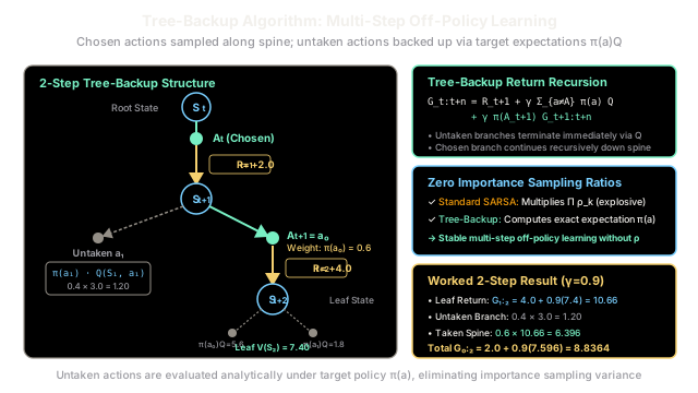
The tree-backup algorithm enables multi-step off-policy reinforcement learning without unstable importance sampling ratios. At each step along a trajectory, untaken actions contribute their expected value under the target policy, while the chosen action carries the multi-step return deeper down the tree.
Why Does This Exist?
In off-policy reinforcement learning, an agent collects experience by behaving according to an exploratory behavior policy , while striving to learn the optimal action-value function or evaluate a distinct target policy .
When extending off-policy methods to multi-step horizons, classical algorithms encounter severe mathematical roadblocks:
- Importance-Sampled -Step SARSA explodes in variance: Standard multi-step off-policy SARSA corrects for the mismatch between behavior and target distributions by multiplying importance sampling ratios along the trajectory: When the target policy differs significantly from , these chained product ratios either collapse to zero (discarding informative multi-step experience) or explode to massive values (inducing devastating sample variance that causes value estimates to diverge).
- Watkins's prematurely terminates traces: Watkins's resolves the off-policy dilemma by zeroing out eligibility traces whenever the agent executes an exploratory (non-greedy) action. In environments requiring continuous exploration, traces are severed after only one or two steps, effectively degrading the multi-step algorithm back into slow, single-step Q-learning.
The Tree-Backup algorithm (introduced by Precup, Sutton, and Singh) solves this fundamental dilemma by achieving multi-step off-policy learning with zero importance sampling ratios.
Instead of adjusting an entire trajectory with multiplicative weights after the fact, Tree-Backup views credit assignment as an explicit decision tree. At each visited state along the trajectory, untaken candidate actions are evaluated analytically using their expected value under the target policy . Meanwhile, the single action that was actually taken continues down the spine to sample future transitions.
By taking exact expectations over unchosen actions, Tree-Backup eliminates importance sampling ratios entirely, providing stable, bounded multi-step credit assignment across arbitrary behavior policies.
Think of It Like This
The Executive Board Decision Audit
Imagine an independent auditor evaluating a regional director's multi-quarter capital allocation decisions.
In Quarter 1, the director faced two options: invest in Project A (a core commercial product with a 60% standard allocation target) or Project B (an experimental venture with a 40% target). The director decided to fund Project A, generating an immediate initial return .
An aggressive, naive auditor might evaluate the director using importance sampling: if the director took a rare 5% exploratory gamble, the auditor would multiply that single outcome by twenty to reweight it to company targets. Over multiple quarters, compounding these artificial multipliers would cause performance ratings to swing wildly from millions of dollars in bonuses to catastrophic penalties.
Instead, the board conducts a tree-backup audit:
- For Project B (which was not chosen), the auditors look at verified market forecasts and record its expected book value: . That branch is closed immediately.
- For Project A (which was actually chosen), the auditors inspect what genuinely occurred in the real world in Quarter 2, weighting that empirical path by its target probability ().
- At the final Quarter 2 milestone, the auditors review all remaining potential avenues using standard expected financial projections.
No explosive artificial multipliers are applied. Unchosen branches are closed using expected values, while the chosen path provides grounded empirical data. The audit remains perfectly aligned with the company's intended policy while staying stable and immune to statistical volatility.
Where the analogy stops: Corporate financial decisions often possess hidden macro-economic cross-dependencies across unchosen projects. In Markov Decision Processes, state transitions satisfy the Markov property: conditional on arriving at state , action values are statistically independent of past history, enabling exact mathematical decomposition.
How It Actually Works
The Tree-Backup Return Recursion and Branching Topology
In the Tree-Backup algorithm, updates are computed for state-action pairs . The backup diagram forms a tree where each visited state branches into all available actions.
Consider an agent observing a trajectory:
generated by behavior policy . The agent evaluates this sequence under target policy .
Level 0: (S_t, A_t) ──► Root action node being updated │ ▼ R_{t+1}Level 1: S_{t+1} ┌──┴─────────────────────────┐ │ │ Untaken a ≠ A_{t+1} Chosen A_{t+1} (The Spine) Bootstrapped via Q Sampled deeper into environment Weight: π(a | S_{t+1}) Weight: π(A_{t+1} | S_{t+1}) │ │ ▼ ▼ R_{t+2} [Terminates branch] S_{t+2} ┌────────┴────────┐ ▼ ▼ Leaf a_0 Leaf a_1 Expected value under target policy π1-Step Base Horizon (Expected SARSA)
For a horizon of , the tree backup return from is identical to the target in Expected SARSA:
where:
- is the immediate observed reward.
- is the discount factor.
- is the probability of selecting action in state under the target policy.
- is the current estimated action-value.
Multi-Step Tree-Backup Return ()
For horizons , the tree backup return is defined recursively:
for , where:
- is the expected value of all candidate actions that were not selected at step .
- is the contribution of the single action that was selected, continuing recursively down the sampled trajectory.
- The leaf step at horizon boundary terminates using the complete expected value: (if is a terminal absorbing state, the second summation is identically zero).
Tabular Action-Value Update
Once steps of experience have been observed, the Q-table entry for the root state-action pair is updated:
where is the step-size learning rate parameter.
Why Importance Sampling is Completely Eliminated
In standard off-policy SARSA, the agent must correct for sampling action from behavior policy rather than target policy , requiring multiplication by the importance sampling ratio .
In Tree-Backup, no importance sampling ratio is needed because the expectation over candidate actions is computed explicitly:
- Untaken actions are multiplied directly by their exact target policy weights .
- The taken action's continuation is scaled directly by its target policy weight .
Because every branch is scaled by and all branches sum to , the distribution is mathematically exact.
The Unified Spectrum:
The Tree-Backup algorithm serves as an anchor in the broader unification of multi-step reinforcement learning. Asis et al. (2017) demonstrated that multi-step SARSA (which fully samples the next action, ) and Tree-Backup (which computes expectations over candidate actions, ) can be unified into a continuous spectrum known as , allowing practitioners to dynamically interpolate between sampling and expectation at every step.
Worked numerical calculation
We compute a concrete 2-step Tree-Backup return () for state-action pair .
Trajectory observed:
Parameters:
- Discount factor:
- Learning rate:
- Initial root value:
Available actions at all states: .
State Dynamics:
- Taken action:
- Untaken action:
- Target policy: ,
- Estimated Q-values: ,
State Leaf Dynamics:
- Target policy: ,
- Estimated Q-values: ,
Step 1: Compute Expected Value at Leaf State
At leaf state , we take the expectation across all candidate actions under target policy :
Step 2: Compute 1-Step Return from
Discounting the leaf value and adding observed reward :
Step 3: Compute Expected Value of Untaken Branches at
The action taken at was . The untaken action is :
Step 4: Weight the Chosen Spine Action at
The recursive multi-step return along the chosen branch is weighted by its target probability:
Combining untaken and chosen branches at :
Step 5: Compute Full 2-Step Tree-Backup Return
Adding immediate reward and discounting the combined branches:
Step 6: In-Place Q-Value Update for
With learning rate and prior estimate :
Every step of the computation operates with bounded values without any probability ratios.
Code
from typing import Dict, List, Tuple
def compute_tree_backup_return( rewards: List[float], states: List[str], actions: List[str], action_space: List[str], policy: Dict[str, Dict[str, float]], q_table: Dict[Tuple[str, str], float], gamma: float, start_t: int, n: int,) -> float: """Compute the n-step Tree-Backup return G_{t:t+n} for starting pair (S_t, A_t).
Args: rewards: Sequence of observed rewards [R_{t+1}, R_{t+2}, ...]. states: Sequence of visited states [S_t, S_{t+1}, ..., S_{t+n}]. actions: Sequence of taken actions [A_t, A_{t+1}, ..., A_{t+n-1}]. action_space: Universal discrete action space. policy: Mapping state -> {action -> probability under target policy pi}. q_table: Action-value table mapping (state, action) -> estimated Q-value. gamma: Discount factor in [0, 1]. start_t: Origin time index t. n: Number of backup steps (horizon).
Returns: Calculated scalar multi-step tree-backup return G_{t:t+n}. """ horizon = min(len(rewards), start_t + n)
# 1. Base case: leaf state S_{horizon} expected value over all candidate actions leaf_state = states[horizon] expected_leaf_val = sum( policy[leaf_state][a] * q_table.get((leaf_state, a), 0.0) for a in action_space )
# Return at the final leaf level current_g = rewards[horizon - 1] + gamma * expected_leaf_val
# 2. Fold backward from horizon - 2 down to start_t for k in range(horizon - 2, start_t - 1, -1): s_kplus1 = states[k + 1] a_kplus1 = actions[k + 1]
# Sum expected values of all untaken actions at S_{k+1} untaken_expected_sum = sum( policy[s_kplus1][a] * q_table.get((s_kplus1, a), 0.0) for a in action_space if a != a_kplus1 )
# Chosen action branch weighted by target policy probability pi(A_{k+1} | S_{k+1}) taken_prob = policy[s_kplus1][a_kplus1] taken_branch_val = taken_prob * current_g
# Combine and discount back to step k current_g = rewards[k] + gamma * (untaken_expected_sum + taken_branch_val)
return current_g
# Verification of 2-step Tree Backup matching the numerical walkthroughrewards_seq = [2.0, 4.0]states_seq = ["S0", "S1", "S2"]actions_seq = ["a0", "a0"]actions_all = ["a0", "a1"]
target_pi = { "S0": {"a0": 0.5, "a1": 0.5}, "S1": {"a0": 0.6, "a1": 0.4}, "S2": {"a0": 0.7, "a1": 0.3},}
q_values = { ("S0", "a0"): 4.0, ("S0", "a1"): 2.0, ("S1", "a0"): 5.0, ("S1", "a1"): 3.0, ("S2", "a0"): 8.0, ("S2", "a1"): 6.0,}
# Compute 2-step Tree-Backup return G_{0:2}ret_2step = compute_tree_backup_return( rewards=rewards_seq, states=states_seq, actions=actions_seq, action_space=actions_all, policy=target_pi, q_table=q_values, gamma=0.9, start_t=0, n=2,)
assert abs(ret_2step - 8.8364) < 1e-4
# Apply in-place tabular Q-value updatealpha = 0.2old_q = q_values[("S0", "a0")]new_q = old_q + alpha * (ret_2step - old_q)assert abs(new_q - 4.9673) < 1e-4
print(f"2-Step Tree-Backup Return G_0:2: {ret_2step:.4f}")print(f"Updated Q(S0, a0): {new_q:.4f}")
# -> 2-Step Tree-Backup Return G_0:2: 8.8364# -> Updated Q(S0, a0): 4.9673Watch Out For
Confusing Tree-Backup with Importance-Sampled SARSA
A common pitfall is attempting to apply importance sampling correction ratios to Tree-Backup returns, assuming that all off-policy methods must be scaled by .
The Failure Mode: When developers insert an importance sampling ratio into the Tree-Backup recursion:
they double-correct for the off-policy distribution.
Because Tree-Backup already weights the spine transition by and sums over all untaken actions analytically, adding introduces redundant scaling. If is small, can be extremely large, instantly destroying Tree-Backup's primary benefit: variance-free multi-step off-policy learning.
Concrete Fix:
- Never use importance sampling ratios () in Tree-Backup. The expectation over action probabilities is performed explicitly in the sum:
- Handle Greedy Target Policies Properly: When learning an optimal policy where is deterministic greedy ( and for ), check whether the chosen behavior action was greedy:
- If the agent took the greedy action (), the untaken sum is zero, and the recursion proceeds with weight .
- If the agent took an exploratory action (), , which cleanly terminates the recursion without requiring special conditional branch cuts.
The Quick Version
- The Tree-Backup algorithm enables multi-step off-policy reinforcement learning without using importance sampling ratios.
- At each step along an exploratory trajectory, untaken candidate actions are backed up analytically by their target policy expectation .
- The single chosen action continues down the spine, weighted by its target policy probability times the recursive return.
- Tree-Backup eliminates importance sampling variance explosion and forms the expectation anchor () of the unified multi-step continuum.