Anomaly Detection in Time Series

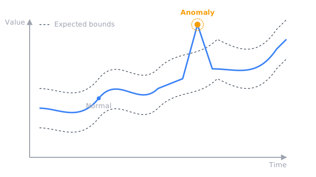
Most points hug a baseline that drifts with trend and season, so subtract what you expect and flag the leftover that is too big to be noise.

A 10.6 spike breaks the 9.58 to 10.42 band around a 10.0 baseline while 10.1 stays inside, so the residual rule flags one point and keeps the other.

Why Does This Exist?

A sensor reports 10.0 all morning, then 10.6 at noon, then 10.1 again. A card stream ticks along, then one charge is forty times the account median. A server fleet hums, then one host stops answering. Each case asks the same question: is this the process, or is this something happening to the process.

The cost of guessing wrong runs both ways. Miss a real break and a forecast trained on the spike bends toward it, so every normal day after looks low. Cry wolf on every wiggle and the on-call team mutes the alert, which is the same as having none. Anomaly detection exists to put that decision on a measured footing instead of a gut threshold on raw values.

This page covers the transient kind: points or short bursts that leave the baseline and come back. A permanent move to a new baseline is a different job and belongs to change point detection. Pulling a series apart into trend, season and leftover so the leftover can be judged fairly is time series decomposition.

Basics first: a residual is the gap between what you expected and what arrived, and everything here keys off that gap. If residuals are new, read the mechanism section below slowly, because the worked example computes each one by hand.

Think of It Like This

The night nurse and the heart monitor

A night nurse watches a heart monitor with the alarm set around the patient resting rate. A reading of 110 means nothing on its own. For a patient asleep at 62, it is a crisis. For the same patient climbing stairs at 105 during physio, it is Tuesday.

The nurse does three things your detector does. First she holds an expectation that moves with context, asleep versus walking, the way your baseline moves with trend and season. Second she judges the gap, not the raw number. Third she has a line where the gap pages someone.

Where it stops: the nurse knows why the context changed, medication, a visitor, a bad dream. Your detector only sees the numbers, so a context shift it was never told about reads as an anomaly. That is why long-lived shifts need change point detection rather than a louder alarm.

How It Actually Works

Call the observed value $y_t$ , the value you expected at that moment $\hat{y}_t$ , and the residual $e_t = y_t - \hat{y}_t$ . Call the typical spread of past residuals $\sigma$ . The score is $z_t = e_t / \sigma$ , the residual measured in units of usual wobble. Flag when $|z_t|$ passes a line like 3.

The baseline moves with the series

A fixed line fails the moment the series has rhythm. Web traffic at noon dwarfs midnight traffic, yet both can be perfectly normal. So the baseline is a moving expectation: a rolling mean, a seasonal naive forecast, or a smoother that knows the hour and the trend. The spread moves too, because a volatile stretch deserves a wider band than a calm one. Judge residuals, never raw values.

The worked example

Five calm readings: $10.0, 10.2, 9.8, 10.1, 9.9$ . Their mean is $50.0 / 5 = 10.0$ , so $\hat{y}_t = 10.0$ . Deviations from the mean are $0, 0.2, -0.2, 0.1, -0.1$ . Squared, those are $0, 0.04, 0.04, 0.01, 0.01$ , summing to $0.10$ . Divide by 5 to get variance $0.02$ , so $\sigma = \sqrt{0.02} \approx 0.1414$ . The 3 sigma band is $10.0 \pm 3 \times 0.1414$ , which is $9.58$ to $10.42$ .

Now two arrivals. First $y_t = 10.6$ : $e_t = 10.6 - 10.0 = 0.6$ , and $z_t = 0.6 / 0.1414 \approx 4.24$ . That clears 3, so flag it. Then $y_t = 10.1$ : $e_t = 0.1$ , and $z_t = 0.1 / 0.1414 \approx 0.71$ . Inside the band, so keep it. Same rule, same band, opposite verdicts, and the diagram above draws exactly this: the 10.6 dot outside, the 10.1 dot inside.

Point, contextual and collective

A point anomaly is off against everything, like the 10.6 above. A contextual anomaly is off only for its slot: 25 degrees is lovely in spring and alarming in a server room at 3 a.m. A collective anomaly is a run where each point looks fine but the shape is wrong, ten slightly-high readings in a row that never individually trip the line. The residual machinery is the same each time. What changes is what the baseline conditions on: nothing, the local context, or the joint shape.

Code

Stdlib only. A rolling mean and spread set the band, then each new point is scored in units of spread:

1import statistics2
3def z_scores(history: list[float], points: list[float]) -> list[float]:4    baseline = statistics.mean(history)5    spread = statistics.pstdev(history)6    return [(p - baseline) / spread for p in points]7
8history = [10.0, 10.2, 9.8, 10.1, 9.9]9print(round(statistics.mean(history), 2))  # -> 10.010print(round(statistics.pstdev(history), 4))  # -> 0.141411print([round(z, 2) for z in z_scores(history, [10.6, 10.1])])  # -> [4.24, 0.71]

The prints are the worked example rerun by machine. A score near 4 trips a 3 sigma line, and a score near 0.7 sleeps through it.

Watch Out For

Alarming on a permanent shift forever

The baseline moves to a new level after a motor wears in or a price tier changes, and every point after reads as anomalous. The symptom is an alert that fires once and never clears: not a spike, a step that stays.

That is not an anomaly problem anymore. Freeze the detector, confirm the regime moved with change point detection, then refit the baseline on the new regime. An anomaly returns to the old line. A shift redraws it.

One global line on seasonal data

Noon traffic equals fifty midnight peaks, so a single threshold on raw values either pages every lunch hour or sleeps through a genuine midnight surge. The symptom is alerts that arrive on schedule, same hour daily, all false.

Fix it by scoring residuals after removing trend and season, the way time series decomposition teaches, or at minimum a rolling window short enough to track the cycle. Bands belong around the expectation, not around the raw series.

The Quick Version

An anomaly is a transient departure from the expected baseline, not a permanent move to a new one.
Judge the residual $e_t = y_t - \hat{y}_t$ , scored as $z_t = e_t / \sigma$ , never the raw value.
Five calm readings averaging 10.0 with spread 0.1414 put the 3 sigma band at 9.58 to 10.42.
A 10.6 arrival scores about 4.2 and gets flagged, while 10.1 scores about 0.7 and is kept.
Context decides the verdict: point, contextual and collective anomalies differ in what the baseline conditions on.
A step that never comes back is a change point, so refit the baseline instead of paging forever.