Change Point Detection

One model stops fitting and two smaller ones fit far better, so cut the timeline where the saving is biggest and start fresh there.

Eight points averaging 8.0 split into means 5.0 and 11.0 cut the squared error from 76 to 4, a saving of 72 no other cut beats.

Why Does This Exist?

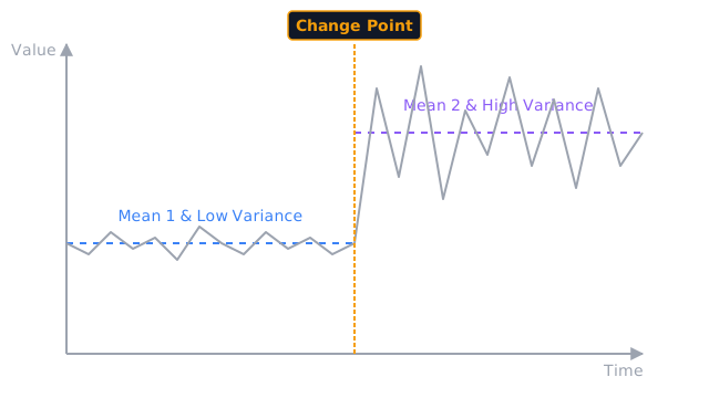
Machines wear in, pricing tiers change, a competitor launches, and the series steps onto a new level for good. A forecaster trained across the step learns a mush average that fits neither side: too high before, too low after. Alerts tuned to the old level either scream forever or sleep through the next real break.

Change point detection exists to cut the timeline where the world changed, so each regime gets its own model, its own baseline, its own honest evaluation. It answers when, not what next, and that when decides which data is even allowed to train the forecaster.

This page covers lasting shifts in the generating process. Brief spikes that return to the old line are anomalies. Measuring an event effect with untreated neighbors alongside is causal inference. Checking whether each regime wobbles around a fixed level is stationarity testing.

Basics first: variance here means squared distance from the segment mean, added up. A segment that hugs its mean is cheap, one that sprawls is expensive, and the whole method is bargain-hunting over cuts.

Think of It Like This

The relay runner swap

You watch one numbered bib circle a track for an hour, but the pace suddenly lifts and stays lifted. Nobody announced a swap, and the bibs all look alike. So you stop watching the runner and watch the splits: the early laps cluster near 90 seconds, the late laps near 75.

One average of 82 seconds describes nobody. Two averages, 90 then 75, describe everybody, and the lap where the description switches is the baton pass. Change point detection is that lap-by-lap accounting done with squared errors instead of a stopwatch.

Where it stops: a single stumbled lap is not a new runner, and cutting there fractures the race into nonsense. Spikes get flagged and ignored per anomaly detection. Cuts are for pace changes that hold.

How It Actually Works

Call a candidate cut $\tau$ (tau) and a cost $C$ that scores how badly one mean fits a stretch. Squared error is the workhorse: $C$ of a segment is the sum of squared gaps from its own mean. The saving from cutting at $\tau$ is:

\text{Saving}(\tau) = C(y_{1:T}) - \left( C(y_{1:\tau}) + C(y_{\tau+1:T}) \right)

A big saving means one mush mean was doing two jobs badly. Each extra cut also pays a penalty, a fixed charge per segment that stops the method from cutting between every pair of points.

The worked example

Eight readings: $[4, 6, 5, 5, 10, 12, 11, 11]$ . Whole mean is $64 / 8 = 8.0$ . Squared gaps: $16, 4, 9, 9, 4, 16, 9, 9$ , summing to $C = 76$ .

Cut after the fourth. Left $[4, 6, 5, 5]$ means $5.0$ with gaps $1, 1, 0, 0$ summing to $2$ . Right $[10, 12, 11, 11]$ means $11.0$ with gaps $1, 1, 0, 0$ summing to $2$ . Post-cut cost $2 + 2 = 4$ , saving $76 - 4 = 72$ .

Cut after the second instead: left $[4, 6]$ costs $2$ , right $[5, 5, 10, 12, 11, 11]$ means $9.0$ and costs $50$ , total $52$ , saving only $24$ . The true seam pays triple the runner-up, which is why the algorithm picks it without hesitation. The diagram draws exactly this split: mean lines at 5.0 and 11.0, cost falling 76 to 4.

Finding the cuts without trying everything

Trying every subset of cuts doubles with each point, so search is the second half of the method. Binary segmentation grabs the single best cut, then recurses left and right: fast and greedy, occasionally fooled. PELT plans all cuts at once with dynamic programming and prunes hopeless branches, reaching the penalized optimum in linear time on well-behaved series. Streaming settings use online variants that test each arrival against the running regime and sound the change within a few points of delay.

Code

Stdlib only. Score every possible single cut by its saving and keep the best:

1def sse(segment: list[float]) -> float:2    mean = sum(segment) / len(segment)3    return sum((v - mean) ** 2 for v in segment)4
5y = [4.0, 6.0, 5.0, 5.0, 10.0, 12.0, 11.0, 11.0]6whole = sse(y)7best = max(8    ((whole - (sse(y[:k]) + sse(y[k:])), k) for k in range(1, len(y))),9)10print(round(whole, 1))  # -> 76.011print(round(sse(y[:4]) + sse(y[4:]), 1))  # -> 4.012print(round(best[0], 1), best[1])  # -> 72.0 4

The machine confirms the hand arithmetic: total 76, best split cost 4 at position 4, saving 72.

Watch Out For

Cutting spikes instead of regimes

Uncleaned outliers fracture the timeline: the method plants one cut where the spike starts and another where it ends, minting a three-point regime of pure noise. The symptom is clusters of cuts a few points apart with absurd means between them.

Clean first, cut second. Flag transients with anomaly detection, handle them before the search, and require a minimum segment length so a two-point excursion cannot become a regime.

A penalty picked by vibes

Too small a per-cut charge shreds stable history into a dozen meaningless phases. Too large buries a genuine but modest shift, and the mush average survives. The symptom in both cases is a segmentation that surprises nobody except the domain expert, who rejects it instantly.

Sweep the penalty and plot cuts against penalty, then pick the elbow where the count stops collapsing, checking each candidate against known events. There is no universal default, because the charge prices a business trade between false alarms and missed shifts, not a math constant.

The Quick Version

A change point is a lasting move to a new regime, while an anomaly visits and returns.
Score cuts by saving: whole-series squared error minus the two segment errors, minus a per-cut penalty.
Eight points averaging 8.0 cost 76 together and 4 split into means 5.0 and 11.0, saving 72.
The runner-up cut saves only 24, so the true seam wins by a factor of three.
Binary segmentation is fast and greedy, while PELT plans all cuts at once with pruning.
Clean spikes first and tune the penalty against known events, or the timeline fractures into noise.