Autocorrelation in Time Series

Slide a series against itself and score the match at each shift, so the shifts that line up expose the rhythm hiding in the wiggles.

Series 1, 2, 1, 2, 1, 2 shifted by one scores minus 0.83 while a shift of two scores plus 0.67, so the ACF bars alternate down, up, down.

Why Does This Exist?

Shuffle a time series and every histogram stays identical while all forecasting dies. Order is the whole game: today leans on yesterday, this January rhymes with last January. Before fitting anything, you need a number for how much the past predicts the present, and at which delays.

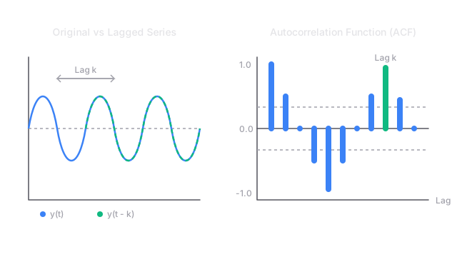
Autocorrelation is that number. Score the series against a delayed copy of itself at each lag, and the pattern of scores tells you what model to reach for. A slow decay across lags means trend, and you should difference first per stationarity testing. A spike at lag 12 in monthly data means yearly season. A clean cutoff after a few lags hands you the memory order for ARIMA. The raw material of the series is time series fundamentals.

Basics first: correlation runs from minus 1 (mirror images) through 0 (no linear link) to plus 1 (lockstep). Autocorrelation is the same idea with the series compared against itself, and a lag is the shift size, so lag 2 compares each value with the one two steps back.

Think of It Like This

The tiled hallway floor

A hallway floor alternates black and white tiles: black, white, black, white down its length. Stand on a tile and look one tile ahead, and you always see the opposite color. Look two tiles ahead, and you always see your own color.

Shift-by-one scores minus, shift-by-two scores plus, and the floor rhythm falls out without measuring a single tile twice. That is all autocorrelation does: step along, compare each position with the one $k$ steps back, and let the agreement at each $k$ name the pattern. A yearly season is the same hallway with twelve tiles per repeat instead of two.

Where it stops: tiles only test straight matching, light against dark. A pattern where the sign flips in a curved or conditional way can score near zero at every shift and still be perfectly predictable, because correlation only sees straight-line links.

How It Actually Works

Call the series $y_t$ with $t$ running $1$ to $T$ , its mean $\bar{y}$ , and the lag $k$ . The autocorrelation at lag $k$ , written $\rho_k$ , is the Pearson correlation of the series with its own shift:

\rho_k = \frac{\sum_{t=k+1}^{T} (y_t - \bar{y})(y_{t-k} - \bar{y})}{\sum_{t=1}^{T} (y_t - \bar{y})^2}

The top adds up agreement between each value and its partner $k$ steps back. The bottom scales everything so the score lands between minus 1 and plus 1. Lag 0 always scores exactly 1, since anything matches itself perfectly.

The worked example

Take $y = [1, 2, 1, 2, 1, 2]$ . The mean is $9 / 6 = 1.5$ . Deviations alternate $-0.5, +0.5, -0.5, +0.5, -0.5, +0.5$ . Squared, each is $0.25$ , and six of them sum to $1.5$ , which is the denominator for every lag.

At lag 1, pair each value from the second onward with its predecessor: $(2, 1), (1, 2), (2, 1), (1, 2), (2, 1)$ . In deviations that is five products of $(+0.5)(-0.5)$ or $(-0.5)(+0.5)$ , each $-0.25$ , summing to $-1.25$ . So $\rho_1 = -1.25 / 1.5 \approx -0.83$ .

At lag 2 the pairs are $(1, 1), (2, 2), (1, 1), (2, 2)$ , four products of $(-0.5)(-0.5)$ or $(+0.5)(+0.5)$ , each $+0.25$ , summing to $1.0$ . So $\rho_2 = 1.0 / 1.5 \approx 0.67$ . Opposite tiles at shift one, matching tiles at shift two, exactly as the hallway promised. Continuing gives $\rho_3 \approx -0.50$ , $\rho_4 \approx 0.33$ and $\rho_5 \approx -0.17$ , the alternating bars drawn in the diagram.

Reading the plot and its bands

An ACF plot draws one bar per lag, and no bar means anything until the sample size backs it. With $T$ points the rough no-signal band sits at $\pm 1.96 / \sqrt{T}$ . Here $T = 6$ , so the band is $\pm 1.96 / \sqrt{6} \approx \pm 0.80$ . Only lag 1 at $-0.83$ peeks outside, which is the plot telling you the honest truth: six points barely support any claim, and the one-shift flip is the only effect big enough to show through.

Code

Stdlib only. The same denominator serves every lag, and each numerator walks the shifted pairs:

1def acf(series: list[float], lag: int) -> float:2    mean = sum(series) / len(series)3    denom = sum((v - mean) ** 2 for v in series)4    numer = sum(5        (series[t] - mean) * (series[t - lag] - mean)6        for t in range(lag, len(series))7    )8    return numer / denom9
10y = [1.0, 2.0, 1.0, 2.0, 1.0, 2.0]11print(round(acf(y, 0), 2))  # -> 1.012print(round(acf(y, 1), 2))  # -> -0.8313print(round(acf(y, 2), 2))  # -> 0.67

Three prints matching the hand computation above, including the perfect self-match at lag 0.

Watch Out For

Reading lag 4 through lags 1 to 3

Lag 4 looks meaningful, but each step echoes the last, so some of that score rode in through the intermediate shifts rather than jumping directly. The symptom is a long smear of decaying bars where every lag looks important and no order can be picked.

The direct effect at each lag is the partial autocorrelation function, PACF, which strips out the shorter shifts first. Use ACF to spot season spikes and PACF to pick the ARIMA memory order. One shows the echo including relays, the other shows each lag own voice.

Trusting bars the sample cannot support

Six points give a band of $\pm 0.80$ , so a bar at $0.67$ is theater, not signal: only two to four pairs sit behind the far lags. The symptom is a confident story about lag 5 built from a single pair of points.

Check the $\pm 1.96 / \sqrt{T}$ bands before reading any bar, and distrust far lags where few pairs overlap. When the bands swallow everything, collect more history or difference the trend away per stationarity testing instead of narrating noise.

The Quick Version

Autocorrelation scores a series against its own delayed copy at each lag, from minus 1 to plus 1.
Series 1, 2, 1, 2, 1, 2 has mean 1.5 and scores minus 0.83 at lag 1 and plus 0.67 at lag 2.
Lag 0 always scores 1, because any series matches itself with no shift.
With 6 points the no-signal band is about plus or minus 0.80, so only lag 1 clears it here.
Slow decay across lags means trend, and a lone spike at the season length means seasonality.
Partial autocorrelation strips relay effects out, and it is the one that sets model memory order.