Decomposing Time Series Into Parts

One sales number hides three stories. Split it into slow trend, repeating season, and leftover noise to see which one moved.

Twelve splits into trend 8 plus season 3 plus leftover 1, so the spike reads as season not surprise

Why Does This Exist?

A weekly total of 12 looks simple until you must act on it. Is 12 high because business grows, because this week always runs hot, or because something odd happened once? The raw number cannot answer. A forecaster that learns raw totals mixes all three, and an alert on raw totals fires every busy season.

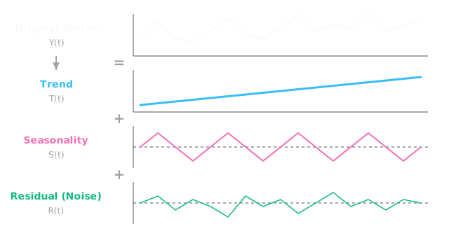
Decomposition untangles them. Trend $T_t$ carries the slow level. Season $S_t$ carries the calendar. Leftover $R_t$ carries the surprise. Forecast trend and season separately, then judge leftovers for anomalies. That split also steadies modelling, because each part is simpler than the mix.

This page teaches the split and the two combining rules. The calendar half in detail lives in seasonality and trends. Testing whether the mix is steady lives in stationarity testing. Reading leftovers for alerts lives in anomaly detection.

Basics first: $y_t$ means the observed value at time $t$ . If ordered data is new, read time series fundamentals first. Everything below builds on why order matters.

Think of It Like This

One cafe song split into three tracks

You hear one song in a busy cafe. The recording actually holds three tracks. The bassline climbs slowly through the verse. The drums hit the same pattern every bar. The crowd and static crackle with no pattern at all.

The bassline is trend. The drums are season. The crowd is leftover noise. Solo each track and you hear its job clearly.

Where it stops: a mixing desk made those tracks separately. A real series arrives already mixed, so every split is an estimate. Change the method and the trend shifts a little, which never happens with true studio tracks.

How It Actually Works

Decomposition assumes $y_t$ combines three parts. Call $T_t$ the trend-cycle, meaning the slow level if seasons vanished. Call $S_t$ the seasonal part, meaning the calendar offset with fixed period $m$ . Call $R_t$ the residual, meaning what trend plus season cannot explain.

Two combining rules cover most data:

Additive says $y_t = T_t + S_t + R_t$ . Use it when seasonal swings hold about the same units as the level rises.
Multiplicative says $y_t = T_t \times S_t \times R_t$ . Use it when swings grow in proportion, like a holiday lift of 25 percent rather than 30 units.

The classical build runs in three passes. First estimate trend with a centered moving average whose window equals $m$ , so one full season cancels itself. Then remove trend by subtraction for additive or division for multiplicative, and average each calendar position across years to kill noise and keep season. Three Januarys detrended to 3, 4, and 2 average to $(3 + 4 + 2) / 3 = 9 / 3 = 3$ . Finally remove trend and season to leave residuals. Modern STL swaps the moving average for local regression, so season can drift slowly instead of repeating rigidly.

Worked example

One week reads 12. The split says trend 8 plus season 3 plus leftover 1.

Check: $8 + 3 + 1 = 12$ . The parts rebuild the total exactly.
The spike is season, not surprise. Expected level with season is $8 + 3 = 11$ , so the true surprise is only $12 - 11 = 1$ .
Alert on raw 12 and you chase a normal busy week. Alert on leftover 1 and you stay quiet.

Push the same shop two years forward with doubled level. If December still adds 3 units, stay additive. If it now adds 6, the swing doubled with trend, so switch to multiplicative or log before you trust the split.

Code

This stdlib snippet checks the additive split and recovers one seasonal position by averaging, the same arithmetic as above:

1def check_additive(y: float, trend: float, season: float, resid: float) -> float:2    """Rebuild the observed value from its three parts."""3    return trend + season + resid4
5
6def seasonal_position(detrended: list[float]) -> float:7    """Average one calendar position across years to wash out noise."""8    return sum(detrended) / len(detrended)9
10
11print(check_additive(12.0, 8.0, 3.0, 1.0))  # -> 12.012print(seasonal_position([3.0, 4.0, 2.0]))  # -> 3.013print(12.0 - (8.0 + 3.0))  # -> 1.0

Three calls, one story. The parts sum to 12.0, January averages to 3.0, and the leftover surprise is only 1.0. When the rebuild misses, your rule or your period is wrong.

Watch Out For

Adding what actually multiplies

You decompose exponential shop growth additively. The symptom is a fan in the leftovers: early residuals scatter around zero, later ones swing wider each year, with December always high. You tuned the season twice and the fan stays.

Fix it by comparing swing height to level. If both double together, move to multiplicative or log the series first. Additive on multiplicative data manufactures fake anomalies every peak season.

Freezing a season that drifts

You use classical averages while shopping habits shift earlier each year. The symptom is season leaking into leftovers: residuals show a calendar shape instead of hash, and last year season misfires this year.

Fix it by letting season evolve with STL or a seasonal model that updates. Classical decomposition assumes the same January forever. When behaviour moves, that assumption becomes the error.

The Quick Version

Decomposition splits $y_t$ into trend plus season plus leftover noise.
Twelve equals trend 8 plus season 3 plus leftover 1, so the surprise is only 1.
Additive adds units. Multiplicative scales with level.
Average each calendar slot across years to isolate season from noise.
Judge spikes in leftovers, not in raw totals.
Let season drift with STL when habits move, or leftovers inherit the calendar.