ARIMA Models

Difference the series until its mean sits still, then forecast the next step from recent values plus recent mistakes.

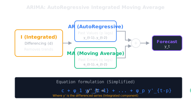
Series 5, 7, 9 and 11 differences into steady 2s, then 0.6 times the last step plus 0.3 times the last error forecasts 12.32 next.

Why Does This Exist?

Two facts about the near future are usually predictive: where the series just was, and where your last forecast just missed. Autoregression uses the first. A moving average over past errors uses the second. Both assume the series wobbles around a fixed level, which real series rarely do because trends drag the level along.

ARIMA exists to bundle the fix with the forecast. Difference the series until its mean sits still, fit the value-and-error regression on that steadied series, then undo the differencing to land back on the original scale. It is the baseline every fancier forecaster must beat, and when it wins, the lesson is that the series was mostly momentum plus noise.

This page covers the non-seasonal model picked by orders $p$ , $d$ and $q$ . Seasonality with its own extra orders lives in sarima. Whether the series is steady enough to model at all is the stationarity question, and the lag diagnostic that sets $p$ and $q$ is autocorrelation.

Basics first: a lag is just how many steps back you look, so lag 1 means yesterday. Stationarity means the mean and spread stay put over time. Everything below assumes those two ideas and links them where used.

Think of It Like This

The delivery van on a hill

You drive a van across a hilly town and log the odometer each minute: 5, 7, 9, 11 kilometres. Predicting the raw odometer is silly because it always climbs. Predicting the per-minute gain is easy, because the gains sit still at 2.

That is differencing: stop forecasting the climbing total and forecast the steady step. Then two corrections steer you. The van keeps its speed, so most of the last step carries forward, and that is the autoregressive part. Your last guess overshot a pothole, and part of that miss carries into the next minute, which is the moving average part. ARIMA is the habit of forecasting gains with both corrections, then adding the gain back onto the odometer.

Where it stops: hills change. A new gradient means a new typical step, and no fixed blend of old steps tracks it. That drift is why the stationarity check comes before the model, not after.

How It Actually Works

Name the series $y_t$ , the value at time $t$ . Name the differenced series $y'_t = y_t - y_{t-1}$ , the step from the last value. Name past mistakes $\varepsilon_t$ , the gap between forecast and truth. The orders are $p$ for how many past steps feed the forecast, $d$ for how many times you difference, and $q$ for how many past mistakes feed it.

Difference first, then regress

With $d = 1$ , model the steps $y'_t$ instead of the levels $y_t$ . A steady climb becomes a flat line of equal steps, and a flat line has the fixed mean the regression needs. If the steps still drift, difference again, but each round costs one observation and injects noise, so stop at the first order that steadies the mean.

One equation with two memories

An ARIMA( $p$ , $d$ , $q$ ) forecast of the next steadied value blends both memories:

y'_t = c + \phi_1 y'_{t-1} + \dots + \phi_p y'_{t-p} + \theta_1 \varepsilon_{t-1} + \dots + \theta_q \varepsilon_{t-q} + \varepsilon_t

Here $c$ is a constant drift, each $\phi$ (phi) weights a past step, and each $\theta$ (theta) weights a past mistake. Set all $\theta$ terms to zero and the model trusts momentum only. Set all $\phi$ terms to zero and it trusts only the correction of old misses. Then integrate: add the predicted step back onto the last level to return to $y_t$ .

Worked example

Take $y = [5, 7, 9, 11]$ . First differences: $7 - 5 = 2$ , $9 - 7 = 2$ , $11 - 9 = 2$ , so $y' = [2, 2, 2]$ . Steady, so $d = 1$ suffices.

Fit ARIMA(1, 1, 1) with $\phi_1 = 0.6$ , $\theta_1 = 0.3$ , and last recorded mistake $\varepsilon_{t-1} = 0.4$ . The next step forecast is $0.6 \times 2 + 0.3 \times 0.4 = 1.2 + 0.12 = 1.32$ . Add it back: $11 + 1.32 = 12.32$ . Momentum alone would have said $11 + 1.2 = 12.2$ , and the error correction nudges it to 12.32. The diagram above draws this exact lane: 5, 7, 9, 11 across the top, 2, 2, 2 below, 12.32 at the end.

Code

Stdlib only. Difference the levels, blend the last step with the last recorded miss, integrate back:

1def diffs(levels: list[float]) -> list[float]:2    return [levels[i] - levels[i - 1] for i in range(1, len(levels))]3
4levels = [5.0, 7.0, 9.0, 11.0]5steps = diffs(levels)6forecast_step = 0.6 * steps[-1] + 0.3 * 0.47print(steps)  # -> [2.0, 2.0, 2.0]8print(round(forecast_step, 2))  # -> 1.329print(round(levels[-1] + forecast_step, 2))  # -> 12.32

Three prints, three claims from the worked example, each reproducible without any statistics library.

Watch Out For

Differencing a series that was already steady

The steps start alternating plus, minus, plus around zero and lag 1 autocorrelation dives toward negative 0.5. The symptom is a model that was fine at $d = 0$ and got worse at $d = 1$ , with the moving average term working overtime to cancel the damage.

Each difference manufactures a zigzag the model must then unlearn. Difference to achieve a steady mean, confirmed by the stationarity check, and stop there. In practice $d$ above 2 is a smell, not a setting.

Ordering seasonality with non-seasonal knobs

A monthly series spikes every December and $p = 11$ starts looking tempting. The symptom is a long tail of significant lags at 12, 24, 36 that no small $p$ or $q$ absorbs without dozens of parameters.

That rhythm needs seasonal orders, not bigger $p$ . Reach for sarima, which differences at lag 12 and adds seasonal memory on top of this page machinery. Let ARIMA own the short memory and give the calendar its own terms.

The Quick Version

ARIMA forecasts the next value from recent steps plus recent mistakes, after differencing the series steady.
Orders $p$ , $d$ and $q$ count past values used, differencing rounds applied, and past errors used.
Series 5, 7, 9 and 11 differences once into steady 2s, so $d = 1$ is enough.
With weights 0.6 and 0.3 and a last miss of 0.4, the next step is 1.32 and the next level is 12.32.
Momentum alone would call 12.2, so the 0.12 nudge is the error memory doing its only job.
Differencing past steadiness injects fake zigzag, and calendar rhythm needs seasonal orders instead.