Causal Inference in Time Series

Before-and-after lies whenever trend or season moves on its own, so build the world without the event and measure against that instead.

Controls at 24 and 25 project a counterfactual of 34 and 35 while actuals print 39 and 41, leaving pointwise lifts of plus 5 and plus 6.

Why Does This Exist?

A campaign launches, sales jump 15 percent, and the team celebrates. Then someone asks whether November always jumps 15 percent, and the room goes quiet. Before-and-after comparisons take credit for every trend, season and market swing that happened to coincide with the event.

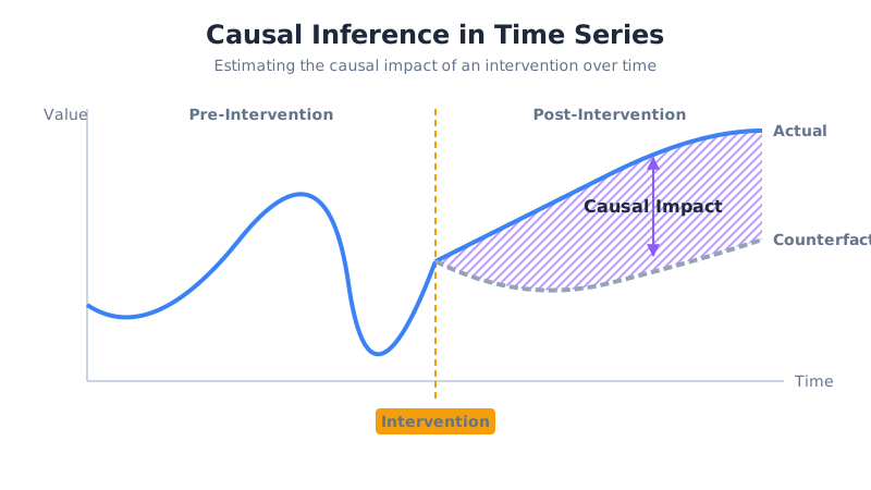
Causal inference in time series exists to price the event honestly. Split history at the intervention, learn how the target moved with untouched controls before it, project that relationship forward as the world-without-the-event, and subtract. What remains is the event own contribution, with uncertainty attached instead of applause.

This page covers the counterfactual build for a single treated series with control series alongside. A permanent level or variance move with no controls to lean on is a change point detection problem. Single spikes that return to baseline are anomalies. The vocabulary of trends and seasons used throughout is time series fundamentals.

Basics first: a counterfactual is the unobserved twin of history, what would have printed had the event never happened. A control series is an untreated neighbor that dances to the same market music. Everything below builds the first from the second.

Think of It Like This

Two shops on one street

Two coffee shops share a street, the same weather, the same foot traffic, the same payday rhythms. Yours refits the window in June. Theirs does not. July sales rise in both shops, because summer lifts the whole street, but yours rises more.

The neighbor is your counterfactual donor. Their July tells you what your July would have looked like with the old window: your June gap over theirs, carried forward. The extra rise above that projection is the window doing, and the street-wide summer lift is correctly left out of its bonus.

Where it stops: if your new window is so striking that passers-by skip the neighbor and come to you, their sales sag and your projection sags with them. A control the treatment touches stops being a control, and the lift estimate quietly shrinks toward zero.

How It Actually Works

Call the treated series $Y_t$ and the untouched controls $X_t$ . Call the intervention time $T_0$ . Fit the relationship on $t < T_0$ , freeze it, feed it the post-event controls, and read off the counterfactual $\hat{Y}_t$ . The pointwise effect is $\Delta_t = Y_t - \hat{Y}_t$ , actual minus would-have-been. Sum $\Delta_t$ for the cumulative lift.

Learn the partnership before the event

On pre-event data, model the target from the controls plus trend and season: $Y_t = f(X_t) + \text{trend}_t + \text{season}_t + \varepsilon_t$ . The controls absorb market-wide moves, the components absorb the calendar, and the leftover $\varepsilon_t$ should look like noise. If the model cannot track the target before the event, its after-the-event projection is fiction, and no wider interval fixes that.

Project, then subtract

After $T_0$ , push the actual control values through the frozen model. Controls must be genuinely untreated here: same market, zero exposure. The output path with its band is the synthetic counterfactual. Each gap between actual and path is one $\Delta_t$ , and the band widths say how seriously to take it.

Worked example

Pre-event, the treated city runs exactly 10 above its control: controls $[20, 22, 21, 23]$ , treated $[30, 32, 31, 33]$ . The learned rule is $\hat{Y}_t = X_t + 10$ .

Post-event controls print $[24, 25]$ , so the counterfactual is $[34, 35]$ . Actual treated sales print $[39, 41]$ . Pointwise lifts: $39 - 34 = 5$ and $41 - 35 = 6$ . Cumulative lift $5 + 6 = 11$ , average $5.5$ per week. A naive before-and-after would compare 41 against a pre average of 31.5 and claim nearly 10, pocketing the market rise the controls reveal. The diagram draws exactly this: two paths parting at the event line, gaps marked plus 5 and plus 6.

Code

Stdlib only. The rule learned pre-event is carried forward onto post-event controls, then subtracted:

1pre_control = [20.0, 22.0, 21.0, 23.0]2pre_treated = [30.0, 32.0, 31.0, 33.0]3gap = sum(t - c for t, c in zip(pre_treated, pre_control)) / len(pre_control)4
5post_control = [24.0, 25.0]6actual = [39.0, 41.0]7counterfactual = [c + gap for c in post_control]8effects = [a - e for a, e in zip(actual, counterfactual)]9print(counterfactual)  # -> [34.0, 35.0]10print(effects)  # -> [5.0, 6.0]11print(sum(effects))  # -> 11.0

The machine repeats the hand arithmetic: projection 34 and 35, lifts 5 and 6, cumulative 11.

Watch Out For

Controls the treatment quietly reached

The campaign spills into the control city through national search ads, or the treated shop steals the neighbor foot traffic. The symptom is a counterfactual that bends toward the actuals, so a real lift reads as plus 1 instead of plus 5, with tight bands that look reassuring.

Audit exposure before modeling, not after. Map every channel the treatment could travel, delivery zones, shared auctions, word of mouth, and drop any control it touches. One clean control beats five clever but tainted ones.

A pre-period too short to learn the rhythm

Two weeks of history cannot teach yearly season or payday cycles, so the frozen model projects a flat line through a seasonal wave. The symptom is a counterfactual that misses the pre-period own shape, with post-event gaps that mirror the calendar rather than the event.

Keep several full cycles of pre-event data, ideally three to four times the evaluation window. Check the fit where truth exists, before the line, and only then trust it where truth does not.

The Quick Version

Before-and-after credits the event with trend and season, so build the untreated twin and subtract that instead.
The counterfactual is the frozen pre-event model fed with post-event control values.
Controls at 24 and 25 project 34 and 35, while actuals of 39 and 41 leave lifts of plus 5 and plus 6.
Cumulative lift is 11 over two weeks, against a naive before-and-after claim of nearly 10 in one.
Controls must be untreated and the pre-period long enough to learn the rhythm, or the gaps lie.
A permanent shift with no controls to borrow is a change point problem, not a causal one.