Time Series Cross-Validation

Shuffled folds let a forecast cheat by training on the future. Walk-forward splits train only on the past and test only on what comes next.

Expanding windows train only on rows before each test block, so the honest error is 2.40 while a shuffled split leaks to 0.45

Why Does This Exist?

You need an error number you can trust before a forecast ships. Ordinary k-fold shuffles the rows, so one fold trains on March and December and validates on June. The model interpolates between future and past it will never have together in production, and the error comes back small and meaningless.

Time series cross-validation exists to enforce one rule: every test block sits strictly after every row used to train it. That simulates deployment, where you stand in the present with only the past in hand. Without it, every metric lies, no matter how carefully the metric itself is chosen.

This page covers the split mechanics: expanding windows, sliding windows, and the production schedule called walk-forward validation. Scoring those splits with MAE or RMSE belongs to evaluation metrics. Turning history into columns the model can read belongs to feature engineering.

Basics first: ordered rows break the independent samples assumption behind shuffling. If that break is new, read time series fundamentals first. Everything below assumes you know why tomorrow depends on today.

Think of It Like This

Weekly quizzes taken in order

A student takes weekly quizzes through a textbook. Fair grading lets quiz 5 use only chapters 1 to 4. Quiz 6 may then use chapters 1 to 5, because chapter 5 has now been taught and tested.

Shuffle the chapters into random piles and quiz 5 gets built with chapter 8 answers inside it. Of course the score looks strong. It studied the ending before taking the middle test.

Expanding windows keep every past chapter. Sliding windows keep only the last three chapters and drop older ones when the syllabus drifts. The production schedule, walk-forward validation, simply repeats the real routine: study, quiz, advance one week, repeat.

Where it stops: textbook chapters stay fixed once printed. Real processes drift, break, and shift level, so a split that was fair last quarter can still straddle a break this quarter.

How It Actually Works

Call the series $y_t$ , meaning the value at time $t$ . Call the training block the rows the model fits, and the test block the later rows it scores. Call $h$ the horizon, meaning how many steps ahead each test block reaches. The rule is positional: the largest training index is always smaller than the smallest test index.

Expanding and sliding windows

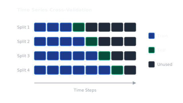
An expanding window anchors the start at the first row and grows the end. Fold one trains on rows 0 to 4 and tests row 5. Fold two trains on rows 0 to 5 and tests row 6. Each fold uses more history, which suits a stable process.

A sliding window fixes the training length and moves both ends. Fold one trains on rows 0 to 4 and tests row 5. Fold two trains on rows 1 to 5 and tests row 6. Old rows drop out, which matches the data volume production will have and adapts faster when the process drifts.

Walk-forward validation is the same mechanic run at deployment granularity: retrain on schedule, predict the next block of length $h$ , record the score, advance, and repeat. Leave a gap between train and test when production has retraining delay, so the split cannot use rows that will not be ready in time.

Worked example

Twelve readings: $10.0$ , $12.0$ , $11.0$ , $13.0$ , $12.0$ , $14.0$ , $13.0$ , $15.0$ , $14.0$ , $16.0$ , $15.0$ and $28.0$ , with a level shift at the end. Score index 5, whose true value is $14.0$ , with a mean-of-training predictor.

The expanding window trains on indices 0 to 4, the only rows a real forecast could have seen. Their values are $10.0$ , $12.0$ , $11.0$ , $13.0$ and $12.0$ . Their sum is $58.0$ and their mean is $58.0 / 5 = 11.60$ . The absolute error against $14.0$ is $|11.60 - 14.0| = 2.40$ .

The shuffled split trains on every other row, including the later $15.0$ , $16.0$ and the $28.0$ spike. Those eleven values sum to $159.0$ with mean $159.0 / 11 = 14.45$ . The error against $14.0$ is $|14.45 - 14.0| = 0.45$ .

Same predictor, same validation point, yet the shuffled error is more than five times smaller. The gap is borrowed information: future rows pulled the mean toward the answer. That is the diagram: three growing train blocks with later test blocks, and the future strictly blocked.

Code

The point is the comparison: one mean predictor, two training sets, and the leaked one wins by cheating.

1series: list[float] = [10.0, 12.0, 11.0, 13.0, 12.0, 14.0, 13.0, 15.0, 14.0, 16.0, 15.0, 28.0]2
3
4def mean(ids: list[int]) -> float:5    return sum(series[i] for i in ids) / len(ids)6
7
8exp_train: list[int] = [0, 1, 2, 3, 4]9val: int = 510shuf_train: list[int] = [i for i in range(len(series)) if i != val]11
12m_exp: float = mean(exp_train)13m_shuf: float = mean(shuf_train)14print(f"expanding mean {m_exp:.2f} err {abs(m_exp - series[val]):.2f}")15# -> expanding mean 11.60 err 2.4016print(f"shuffled mean {m_shuf:.2f} err {abs(m_shuf - series[val]):.2f}")17# -> shuffled mean 14.45 err 0.45

The honest 2.40 predicts deployment. The flattering 0.45 predicts only the leak.

Watch Out For

Scaling the whole series before splitting

You standardize all twelve readings at once, then run the expanding splits. The mean and variance used on fold one already contain the later 28.0 spike, so training rows carry future information even though the indices look clean.

Symptom: honest splits still report small errors that collapse in production. Fix: fit every scaler, imputer, and feature transformer inside each training block only, then apply it to that fold test block. Treat any transformer fit on the full series as a leak.

Testing with no gap when production has delay

Your pipeline needs two days to retrain, but each split tests the very next row. The split measures a reaction speed production cannot achieve.

Symptom: backtest errors look better than live errors by a stable margin, concentrated at turning points. Fix: insert a gap of the retraining delay between train end and test start, and set the step size and horizon $h$ to the real deployment cycle. A weekly deployment forecasting 14 days ahead validates in 7-day steps with a 14-day horizon.

The Quick Version

Every test block must sit strictly after every row that trained the model scored on it.
An expanding window grows training fold over fold, while a sliding window keeps training length fixed and drops old rows.
Walk-forward validation runs the same mechanic at the schedule production will retrain at, with a gap when retraining has delay.
Twelve readings with a late spike give an honest mean error of 2.40 against a shuffled error of 0.45 on the same point.
Report the trend across folds, not the earliest small-history fold alone.
Scoring the test blocks with MAE or RMSE is a separate choice covered in evaluation metrics.