Time Series Evaluation Metrics

One forecast needs several scores. MAE stays steady, RMSE punishes one big miss, and percentage errors let you compare across scales.

Four forecasts with errors 1, 0, 2 and 3 give MAE 1.50 but RMSE 1.87, because squaring punishes the miss of 3

Why Does This Exist?

A forecast that misses by a little every day and one that nails every day but misses a holiday spike by a mile need different responses. The first wastes a little stock daily. The second empties the shelf on the biggest day of the year. A single average hides which failure you have.

Metrics exist to price errors differently. Some treat every unit the same, some charge extra for large misses, and some divide by the actual value so a pen forecast and a car forecast can share one scoreboard. The split you validate with belongs to cross-validation, which keeps every test block after its training rows. The forecaster you score here is often exponential smoothing.

Basics first: every metric below starts from the residual, meaning actual minus predicted at the same time. If residuals are new, think of them as the signed miss per row before any averaging happens.

Think of It Like This

Darts with two scoring rules

You throw four darts. Three land close to the bullseye and one lands far in the wall.

Mean absolute error measures each throw distance and averages them. Every inch counts the same, so three good throws mostly cover one bad throw.

Root mean squared error squares each distance first. The far throw contributes 9 times more than a throw 3 times farther, so one wild throw decides the score.

Percentage errors judge relative to the target size. Missing by one inch on a dinner plate and on a coin are different achievements, which is why business reports prefer percentages when series live on different scales.

Where it stops: dart throws stand alone, while forecast errors arrive in order and correlate. A metric can price the misses but cannot tell you whether the misses cluster after a break.

How It Actually Works

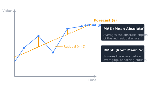
Call the actual at time $t$ by $y_t$ , meaning the observed value. Call the prediction $\hat{y}_t$ , meaning the forecast for that same time. Call the residual $e_t = y_t - \hat{y}_t$ , meaning the signed miss. Call $n$ the count of scored rows.

Mean absolute error averages the absolute miss. It grows linearly, so it stays steady when one outlier appears. $\text{MAE} = \frac{1}{n} \sum_{t=1}^{n} |y_t - \hat{y}_t|$
Root mean squared error averages the squared miss and takes the root, so the units stay original while large misses dominate. $\text{RMSE} = \sqrt{\frac{1}{n} \sum_{t=1}^{n} (y_t - \hat{y}_t)^2}$
Mean absolute percentage error divides each absolute miss by its actual, then averages as a percent. It allows comparison across scales but breaks near zero. $\text{MAPE} = \frac{100}{n} \sum_{t=1}^{n} \left|\frac{y_t - \hat{y}_t}{y_t}\right|$
Symmetric MAPE divides by the average of actual and predicted magnitudes, which softens the asymmetry when actuals vary widely. $\text{sMAPE} = \frac{100}{n} \sum_{t=1}^{n} \frac{|y_t - \hat{y}_t|}{(|y_t| + |\hat{y}_t|)/2}$

Worked example

Actual values $10$ , $12$ , $11$ and $15$ . Predicted values $9$ , $12$ , $13$ and $12$ . Residuals are $1$ , $0$ , $-2$ and $3$ .

Absolute misses are $1$ , $0$ , $2$ and $3$ . Their sum is $6.0$ and $\text{MAE} = 6.0 / 4 = 1.50$ .

Squared misses are $1$ , $0$ , $4$ and $9$ . Their sum is $14.0$ , their mean is $3.50$ , and $\text{RMSE} = \sqrt{3.50} = 1.87$ . The miss of $3$ contributes $9$ of the $14$ squared total, which is why RMSE at $1.87$ sits above MAE at $1.50$ .

Percentage misses are $1/10 = 0.10$ , $0/12 = 0$ , $2/11 = 0.1818$ and $3/15 = 0.20$ . Their mean is $0.1205$ , so $\text{MAPE} = 12.05$ percent.

Symmetric denominators are $9.50$ , $12.0$ , $12.0$ and $13.50$ . The ratios are $0.1053$ , $0$ , $0.1667$ and $0.2222$ . Their mean is $0.1235$ , so $\text{sMAPE} = 12.35$ percent. That is the diagram: four actual and forecast dots with error bars, and the bar of length $3$ highlighted as the RMSE driver.

Code

The point is the gap: same four forecasts, steady MAE beside outlier-driven RMSE, computed with the standard library only.

1actual: list[float] = [10.0, 12.0, 11.0, 15.0]2pred: list[float] = [9.0, 12.0, 13.0, 12.0]3
4abs_err: list[float] = [abs(a - p) for a, p in zip(actual, pred)]5mae: float = sum(abs_err) / len(abs_err)6print(f"{mae:.2f}")  # -> 1.507
8sq: list[float] = [(a - p) ** 2 for a, p in zip(actual, pred)]9rmse: float = (sum(sq) / len(sq)) ** 0.510print(f"{rmse:.2f}")  # -> 1.8711
12mape: float = sum(abs(a - p) / a for a, p in zip(actual, pred)) / len(actual) * 100.013print(f"{mape:.2f}")  # -> 12.0514
15smape: float = sum(abs(a - p) / ((abs(a) + abs(p)) / 2.0) for a, p in zip(actual, pred)) / len(actual) * 100.016print(f"{smape:.2f}")  # -> 12.35

Four prints, four agreements with the hand steps. Change the last prediction from $12$ to $15$ and RMSE falls to meet MAE, which confirms the outlier was driving the gap.

Watch Out For

MAPE on rows that can be zero

Intermittent demand holds many true zeros. MAPE divides by $y_t$ , so one zero actual sends that term toward infinity and the average with it.

Symptom: a forecast that looks sane reports MAPE in the thousands while MAE stays small. Fix: never use MAPE where zeros occur. Report MAE alongside RMSE for scale, or use sMAPE with care, and slice errors by nonzero demand separately.

Reading RMSE alone after a spike

One missed promotion dominates the squared total, so RMSE describes that week rather than the typical week.

Symptom: RMSE far above MAE, here $1.87$ against $1.50$ , with most of the squared sum in one term. Fix: always report both. When they disagree, inspect the largest residuals first, and validate the split itself with cross-validation before tuning the model.

The Quick Version

MAE averages absolute misses and treats every unit the same, here 1.50 on four forecasts.
RMSE squares misses first, so one miss of 3 lifts it to 1.87 on the same rows.
MAPE divides by actuals for scale-free comparison, here 12.05 percent, but breaks on zero actuals.
sMAPE softens asymmetry with averaged denominators, here 12.35 percent.
Report MAE with RMSE together. A gap between them points at a few large errors, not steady bias.
Honest splits come first, so score these metrics only on test blocks after their training rows.