Transformer Forecasting for Series

A transformer reads the whole past window at once. Attention weighs every old step directly, so last winter can speak to this winter.

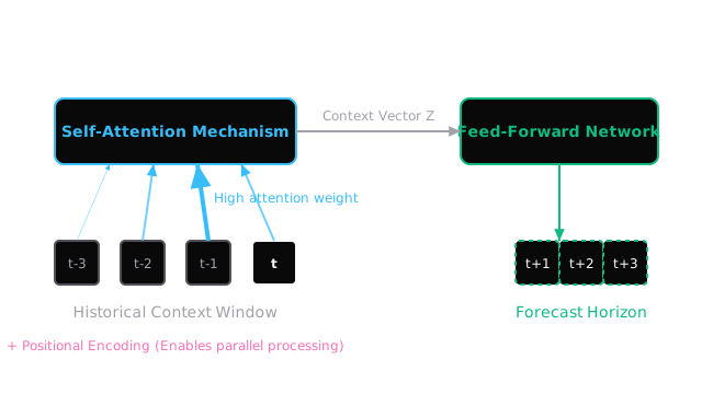
Scores 2 1 0 become weights 0.665 0.245 0.090 and blend 10 12 8 into 10.3 without stepping in order

Why Does This Exist?

Recurrent nets read history in order, one step at a time. That chain is honest but slow, and old steps fade as gradients travel back. By step 200, last season is a whisper. You want a model that asks every past step directly, however far back it sits, and trains in parallel instead of queuing.

Attention does that. It scores every pair of steps, turns scores into weights, and blends the past in one hop. The path from any history point to the forecast stays one hop long. Long seasonal links stop fading, and the whole window trains at once.

This page teaches that swap: patching, position tags, attention, and horizon decoding. The recurrent predecessor lives in LSTM forecasting. The ordered-data base lives in time series fundamentals. Stretching one prediction into many lives in multi-step forecasting. Judging the result lives in evaluation metrics.

Basics first: $L$ means lookback length, $H$ means horizon length, and a token here means one patched chunk of steps. If ordered data is new, read fundamentals first. Everything below assumes you know why shuffling breaks time.

Think of It Like This

Reading front to back versus jumping with search

An LSTM reads like you reading a logbook front to back. By page 200 you remember the gist of page 10, not its numbers. To quote page 10 you walk back through 190 pages.

A transformer reads like you with search over the same logbook. You type one query and jump straight to page 10, compare it with page 200 side by side, and quote both exactly. Distance stops mattering.

Where it stops: search finds words for free. Attention learns its jump weights from data and pays for every pair it scores. That freedom costs memory that grows with the square of the window, which reading in order never pays.

How It Actually Works

Call the window $x_{t-L+1}$ to $x_t$ , meaning the $L$ past values ending now. Call the horizon $H$ , meaning how many steps ahead you must emit. Self-attention builds a query $q$ , key $k$ , and value $v$ per token, scores queries against keys, normalises with softmax, and blends values by those weights. Every token reaches every other in one hop, so the maximum path is $O(1)$ .

Three adaptations make it work on time. Patching groups raw steps into chunks, so $L = 96$ hours becomes 24 patches of 4 and the $O(L^2)$ pair cost falls by 16 times. Position and calendar tags restore order, because attention alone cannot tell shuffled from sorted. You add absolute positions plus hour of day and day of week, so the model sees both place and season. Decoding then emits $H$ : one-shot heads write the whole horizon at once and stay stable, while recursive heads feed each prediction back and drift when early steps err.

Worked example

Window of three values: 10, 12, 8. Scores for the forecast query are 2, 1, 0.

Exponentiate: $e^2 = 7.389$ , $e^1 = 2.718$ , $e^0 = 1.000$ . Sum $= 7.389 + 2.718 + 1.000 = 11.107$ .
Weights: $7.389 / 11.107 = 0.665$ , $2.718 / 11.107 = 0.245$ , $1.000 / 11.107 = 0.090$ . They sum to $1.000$ .
Blend: $0.665 \times 10 + 0.245 \times 12 + 0.090 \times 8 = 6.650 + 2.940 + 0.720 = 10.310$ , so the forecast is about 10.3.
Pair cost is $3 \times 3 = 9$ scores for $L = 3$ . Double to $L = 6$ and pairs quadruple to 36.

No chain carried 10 forward through 12 and 8. The query reached back two steps in one hop because the weight 0.665 said so.

Code

This stdlib snippet runs the diagram arithmetic: softmax of 2 1 0, the blend into 10.3, and the pair count:

1import math2
3
4def softmax(scores: list[float]) -> list[float]:5    """Normalise scores into weights that sum to 1."""6    exps: list[float] = [math.exp(s) for s in scores]7    total: float = sum(exps)8    return [e / total for e in exps]9
10
11def blend(values: list[float], weights: list[float]) -> float:12    """Weighted average of past values by attention weights."""13    return sum(v * w for v, w in zip(values, weights))14
15
16values: list[float] = [10.0, 12.0, 8.0]17weights: list[float] = softmax([2.0, 1.0, 0.0])18print([round(w, 3) for w in weights])  # -> [0.665, 0.245, 0.09]19print(round(blend(values, weights), 2))  # -> 10.3120print(3 * 3)  # -> 9

Weights round to 0.665, 0.245, 0.090 and blend to 10.31. Nine pairs for three steps shows the square law before you scale to hundreds.

Watch Out For

Feeding raw ticks into quadratic attention

You pass 10,000 raw ticks to a plain transformer. The symptom is instant failure: memory explodes, batches shrink to 1, then the run dies with an allocation error. Pairs grow as $L^2$ , so 10,000 steps means 100 million scores per head.

Fix it by shortening $L$ before attention. Patch steps into chunks, sample to a coarser grain, or pick a sparse attention variant. Prove the pair math first: $L$ squared times heads must fit your card.

Dropping the position tags

You embed values but forget order info. The symptom is a model blind to shuffling: permute the window and the forecast barely moves, while season flips go unnoticed. Attention alone is a set tool, not a sequence tool.

Fix it by always adding position plus calendar features. Absolute order plus hour of day and day of week turns the set back into a series. Test the fix by shuffling once: a correct model must change its answer.

The Quick Version

Transformers swap the step-by-step chain for one-hop attention over the window.
Scores 2 1 0 normalise to 0.665 0.245 0.090 and blend 10 12 8 into 10.3.
Patching chunks steps to cut the pair cost, which grows as $L$ squared.
Position and calendar tags restore order that attention alone cannot see.
One-shot heads write the horizon at once, recursive heads feed back and can drift.
Raw high-frequency windows blow memory, so shorten $L$ before you attend.