Dilated Convolution

Dilation spreads a small kernel over a wider area by skipping cells, so one layer sees far without extra weights and without shrinking the image.

A 3x3 kernel at dilation 2 spans 5x5 with the same nine weights, and rates 1, 2, 4 stack to a 15 pixel field.

Why Does This Exist?

Dense tasks such as segmentation need two things at once: wide context (is this pixel road or sidewalk depends on the whole street) and full resolution (the boundary must land on the exact pixel). Pooling gives width by shrinking the map, which destroys the boundaries the task must output. Larger kernels give width by adding weights quadratically.

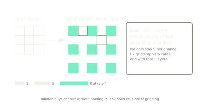
Dilation gives width for free. A 3x3 kernel with dilation rate $r$ spaces its taps $r$ pixels apart, covering $(k-1) \cdot r + 1$ pixels per side with the same 9 weights. This page covers that mechanism and its artifacts. Basic size arithmetic lives in basic CNN operations and field growth in receptive fields.

Think of It Like This

Reading every second fence slat

You stand before a long fence and need its full width without walking. Reading every slat covers little ground. Skipping one slat between reads covers twice the fence with the same number of glances, but you miss whatever hid behind the skipped slats.

Dilation is the skipping. The coverage doubles while the glance count stays fixed, and the missed slats are exactly the gridding artifact described below.

How It Actually Works

Effective kernel span for size $k$ and rate $r$ is $k_{eff} = (k - 1) \cdot r + 1$ . A 3x3 at rate 1 spans 3, at rate 2 spans 5, at rate 4 spans 9. Weight count never moves: $3 \times 3 \times C_{in} \times C_{out}$ regardless of rate.

Stacked dilations add like ordinary kernels. Three 3x3 layers at rates 1, 2 and 4 give spans 3, 5 and 9, and the combined field is $1 + 2 + 4 + 8 = 15$ pixels across from one dimension of stacking. Segmentation backbones use this to hold output stride at 8 instead of 32, keeping 28x28 maps on a 224 input where plain pooling would leave 7x7.

The price is gridding: rate 2 samples a checkerboard, so adjacent output units read disjoint input sets and fine checkerboard detail falls through the gaps. The standard fix stacks coprime rates such as 1, 2 and 5, or ends with two rate-1 layers that fill the holes.

Code

1def span(k, r):2    return (k - 1) * r + 13
4print([span(3, r) for r in (1, 2, 4)])5# -> [3, 5, 9]6
7# stacked receptive field of rates 1, 2, 4 with 3x3 kernels8field = 1 + sum(span(3, r) - 1 for r in (1, 2, 4))9print(field)10# -> 15

Watch Out For

Stacking one dilation rate until gridding appears

Three rate-2 layers in a row sample the same checkerboard at every depth, and thin structures one pixel wide can vanish. The symptom is striped or dotted segmentation on fine detail. Vary rates across layers and finish with rate-1 layers.

Using dilation where downsampling plus a skip would do

Dilation keeps full-resolution maps through the whole network, which costs memory: a 112x112 map holds 16 times the activations of a 28x28 map. When only the final output needs resolution, a strided encoder with a decoder and skips is cheaper than dilating every stage.

The Quick Version

Dilation spaces kernel taps apart so a 3x3 at rate 2 spans 5x5 with the same nine weights.
Span follows effective size (k minus 1) times r plus 1, and stacked fields add.
Segmentation uses it to hold output stride at 8 with wide context and exact boundaries.
Repeated single rates cause gridding artifacts that skip fine detail; vary rates and end with rate 1.
Full-resolution maps cost memory, so dilate the late stages rather than the whole network.