Gamma Correction

Gamma correction raises normalized pixels to a power to undo display nonlinearity, brightening shadows below one and deepening them above one.

A gamma below one lifts the dark end of the curve steeply while barely moving brights, unlike a straight line.

Why Does This Exist?

Screens lie: feeding a display twice the pixel value does not produce twice the light. Cathode physics set a power-law response near $L = V^{2.2}$ , and modern sRGB displays keep a similar curve, while human eyes are most sensitive in shadows. Without compensation, mid-tones render too dark and shadow detail crushes. Gamma correction applies the inverse power law so the end-to-end chain looks linear to the eye. Within enhancement, it is the nonlinear member: gentle in highlights, strong in shadows, the opposite of a straight alpha-beta line.

This page covers the power law, the worked numbers both directions, and the encode-decode pairing everyone confuses.

Think of It Like This

A faucet that gushes at the end

An old faucet barely drips for the first half-turn, then gushes near full open: equal twists give unequal water. Gamma correction is a compensating handle geared in reverse, turning a lot where the faucet gives little and a little where it gushes, so the combined feel is even from closed to open.

The analogy stops at direction. Two opposite handles exist (encoding versus display), and fitting the wrong one doubles the bend instead of straightening it. Labels matter more than with any linear fix.

How It Actually Works

The power law

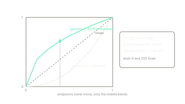
Normalize to $v = r / 255$ in $[0, 1]$ , apply $s = v^{\gamma}$ , rescale to 255. With $\gamma < 1$ the curve bows upward: dark values jump while brights barely move. With $\gamma > 1$ it sags: brights drop fast, shadows compress. Endpoints are fixed (0 stays 0, 1 stays 1), so unlike clipping stretches, gamma never destroys the rails.

Worked both directions on $r = 100$ ( $v = 0.392$ ): brightening with $\gamma = 0.45$ gives $0.392^{0.45} = 0.656$ , times 255 equals 167.3, so the pixel lands at 167, lifted by 67 levels. Darkening with $\gamma = 2.2$ gives $0.392^{2.2} = 0.127$ , times 255 equals about 32.5, so it sinks to 33 after rounding. One input, two opposite fates, set by a single number.

Encode versus display

Cameras encode with $\gamma \approx 1/2.2$ (compressing highlights, expanding shadows for efficient storage); displays decode with $\gamma \approx 2.2$ . The pair multiplies to 1.0 and the image looks right. Applying display gamma to an already-encoded file double-darkens it: the classic "why is my PNG black" bug. Track which side of the chain each array lives on, and convert at capture and display boundaries only.

Fast application

Per-pixel pow over megapixels is slow in Python loops but trivial as a 256-entry lookup table: precompute lut[i] = round(255 \cdot (i/255)^{\gamma}) once and map with cv2.LUT(img, lut). The table also makes the mapping inspectable: plot it and the shadow lift is visible as the steep early slope.

Code

1def gamma_lut_value(r, gamma):2    return round(255.0 * ((r / 255.0) ** gamma))3
4print(gamma_lut_value(100, 0.45))  # lift shadows5# -> 1676print(gamma_lut_value(100, 2.2))  # deepen mid-tones7# -> 33

Watch Out For

Double gamma darkening

Applying a 2.2 curve to an already gamma-encoded image squares the bend and crushes everything below mid-gray to near black. The symptom is a mysteriously dark pipeline output. Check provenance: files from cameras are almost always encoded, so they need decoding (gamma below one) for linear math, not more encoding.

Gamma on raw linear sensor data skipped

Computer vision math (blending, gradients, photometric losses) assumes linear light, but encoded files are nonlinear. The symptom is subtly wrong blends and over-weighted dark-region errors. Linearize with the inverse curve before measuring, and re-encode only for display.

The Quick Version

Gamma maps $s = v^{\gamma}$ on normalized pixels; endpoints never clip.
$\gamma < 1$ lifts shadows (100 becomes 167 at 0.45); $\gamma > 1$ deepens tones (100 becomes 33 at 2.2).
Cameras encode near $1/2.2$ and displays decode near 2.2; the pair cancels.
Apply with a 256-entry lookup table via cv2.LUT for speed.
Linearize before measuring light; encode only for display.