Brightness and Contrast

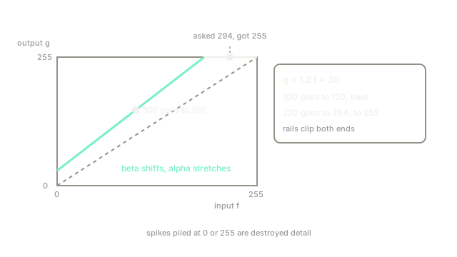
Brightness shifts every pixel by a constant while contrast scales values about the mean, following output equals alpha times input plus beta.

Beta slides the whole histogram sideways for brightness while alpha stretches it wider for contrast, clipping at both ends.

Why Does This Exist?

The two most common image complaints have the simplest fixes: too dark (shift everything up) and too flat (spread values apart). The linear point operation $g = \alpha f + \beta$ does both in one pass and underlies camera exposure compensation, dataset normalization previews, and the first thing every practitioner tries on a dull image. Within the enhancement family, it is the fixed, predictable member: same input always gives same output, unlike histogram methods that vary per image.

This page covers what $\alpha$ and $\beta$ each do, the worked arithmetic, and the clipping both ends pay. For nonlinear shadow lifting, see gamma; for distribution-driven spreading, see histogram equalization.

Think of It Like This

Volume knob and graphic equalizer

Beta is a volume knob: turning it raises every note equally, quiet hiss included. Alpha is the spread control: it pushes loud and soft apart, making the performance punchier but shoving the extremes off the scale into distortion. Both are instant and reversible until clipping hits; once a peak is flattened against the rail, no knob position recovers it.

The analogy stops at color. One knob drives all three channels, so strong settings shift hues as well as lightness: skies go cyan, skin goes orange. Real color work adjusts a luminance channel instead.

How It Actually Works

The alpha-beta equation

For input pixel $f(x, y)$ , output $g(x, y) = \alpha f(x, y) + \beta$ , where $\alpha > 0$ is gain (contrast) and $\beta$ is bias (brightness), computed per channel and clipped to $[0, 255]$ . Here $\alpha$ multiplies distance from black: values spread apart as $\alpha$ grows past 1 and huddle as it drops below 1. $\beta$ adds a constant: the whole histogram slides right for $\beta > 0$ , left for $\beta < 0$ . OpenCV's cv2.convertScaleAbs(img, alpha=1.2, beta=30) does exactly this with saturation built in.

Worked example with $\alpha = 1.2$ , $\beta = 30$ : a mid pixel $f = 100$ becomes $1.2 \cdot 100 + 30 = 150$ , visibly brighter. A bright pixel $f = 220$ asks for $1.2 \cdot 220 + 30 = 294$ , which clips to 255: highlight detail burns out. That pair shows the whole trade in two numbers.

Reading the histogram

Brightness problems show a histogram parked at one end; contrast problems show a narrow hump. After correction the hump should sit centered and wide without piling against either rail. A spike exactly at 0 or 255 is the clipping signature: information destroyed, shown as a wall of pixels the sensor never recorded.

When linear is enough, and when not

Uniform dullness from exposure or lighting surrenders to alpha-beta immediately, and its determinism suits batches and video. It fails on non-uniform defects: one global line cannot lift shadows without blowing highlights in the same frame, and it cannot touch color casts. Those need gamma, CLAHE, or channel-wise work on the color page.

Code

1import numpy as np2
3px = np.array([100, 220])4out = np.clip(1.2 * px + 30, 0, 255).astype(np.uint8)5print(out.tolist())  # alpha=1.2, beta=306# -> [150, 255]

Watch Out For

Clipping disguised as correction

Pushing $\alpha$ and $\beta$ until the image "pops" piles pixels against 0 and 255, erasing texture in shadows and highlights. The symptom is plastic-looking regions with zero gradient. Watch the histogram rails while tuning, and stop before spikes grow.

Hue shifts from channel scaling

Scaling R, G and B by one $\alpha$ changes their ratios, so colors drift as contrast rises. The symptom is blue shadows and sunburned faces after an innocent brightening. For color photos, apply the correction to the V channel in HSV or the L channel in LAB, then convert back.

The Quick Version

$g = \alpha f + \beta$ : $\alpha$ spreads values (contrast), $\beta$ slides them (brightness).
Example: $\alpha = 1.2$ , $\beta = 30$ sends 100 to 150 and clips 220 to 255.
convertScaleAbs computes this with saturation in one call.
Spikes at histogram rails mean destroyed detail, not better contrast.
Correct luminance channels, not raw RGB, to protect hues.