Spatial Attention Masks Where to Look

Spatial attention scores every pixel location for usefulness on this image, then turns up the telling spots and mutes the clutter.

Channel pooling plus a 7 by 7 conv gives gates 0.77 on target and 0.31 on clutter, so the target counts twice as much

Why Does This Exist?

Convolutions share weights everywhere, so a dog ear and a blank wall get equal compute. On cluttered photos the classifier drowns in background votes.

Spatial gates fix that per image. They sit after convolutional layers, complement channel attention which scores what, and lift object detection where location decides.

Think of It Like This

A stage spotlight operator

You watch a dark stage with two actors and empty curtains. You push the spotlight to full on the speaking actor and dim it on the curtains for this scene only.

Maps are the stage, the pooled conv is your eye, and gates are the dimmer. Where it stops: a misaimed spot hides the real action, just as a wrong mask mutes the target.

How It Actually Works

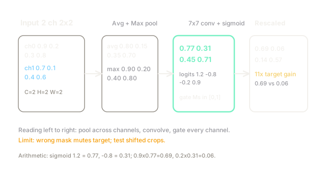
Take feature maps $F$ with shape $C \times H \times W$ , where $C$ counts channels, $H$ height, and $W$ width. Pool across channels two ways at each location $(i,j)$ : average $F_{avg}(i,j)$ and max $F_{max}(i,j)$ . Stack them to $2 \times H \times W$ , run one $7 \times 7$ convolution $f$ , then sigmoid $\sigma$ :

M_s = \sigma(f([F_{avg}; F_{max}]))

$M_s$ is $1 \times H \times W$ with values in $[0,1]$ . Rescale $F' = M_s \otimes F$ , where $\otimes$ multiplies every channel at $(i,j)$ by the same gate $M_s(i,j)$ .

Worked example

Two channels on a $2 \times 2$ map. Channel 0 is $[[0.9, 0.2], [0.3, 0.8]]$ and channel 1 is $[[0.7, 0.1], [0.4, 0.6]]$ . Average pooling gives $[[0.80, 0.15], [0.35, 0.70]]$ since $(0.9+0.7)/2 = 0.80$ and so on. Max pooling gives $[[0.90, 0.20], [0.40, 0.80]]$ .

Say the $7 \times 7$ conv (padded to $2 \times 2$ here) outputs logits $[[1.2, -0.8], [-0.2, 0.9]]$ . Sigmoid gives $[[0.77, 0.31], [0.45, 0.71]]$ because $1/(1+e^{-1.2}) = 0.77$ and $1/(1+e^{0.8}) = 0.31$ . Top-left keeps $0.9 \times 0.77 = 0.69$ while top-right drops to $0.2 \times 0.31 = 0.06$ . The target corner counts eleven times the clutter cell.

Watch Out For

A 7 by 7 gate memorizing training clutter

A large kernel with little data learns dataset corners instead of objects. Symptom: higher train accuracy with worse crops on new scenes. Fix: keep the kernel at $7 \times 7$ with strong image augmentation and check location shift by testing on shifted crops.

The Quick Version

Spatial attention pools across channels to avg and max maps, then conv plus sigmoid makes one gate per location.
Fixture gates 0.77 on target and 0.31 on clutter give an eleven to one emphasis after rescaling.
It scores where, while channel attention scores what, so the pair covers both.
Cost is one small convolution per block, far below self-attention.
Wrong masks mute targets, so test on shifted crops before trusting gains.