Iterative Solvers for Linear Systems

Solve huge systems without factoring: improve a guess step by step, each step costing one matrix-vector multiply. The only option past millions of unknowns.

Two Jacobi iterates step from 0.25 0.667 to 0.083 0.583, visibly homing in on the exact answer 0.091 0.636 without any factorisation

Why Does This Exist?

Direct solvers factor the matrix at $O(n^3)$ . At $n = 10^6$ that is $10^{18}$ operations: over. Yet science and ML routinely solve systems that large (PDE discretisations, graph Laplacians, Hessians). Iterative solvers never factor anything. They hold a guess $x_k$ , spend one matrix-vector multiply to improve it, and stop when the residual is small enough. Cost per step $O(n^2)$ dense, $O(\text{nnz})$ sparse; total cost set by how fast the guesses converge.

Three methods cover the territory. Jacobi updates every coordinate from the old guess simultaneously. Gauss-Seidel reuses fresh values within the sweep, roughly doubling the speed. Conjugate gradient (CG) takes mutually conjugate directions and finishes SPD systems in at most $n$ steps in exact arithmetic, far fewer with clustered eigenvalues. Direct foundations are in linear systems and least squares; the giant-sparse regime continues in sparse matrix methods.

The one idea you need first

The residual $r = b - Ax_k$ measures how far a guess is from solving: zero means done. Iterative methods drive a norm of $r$ down without ever inverting. Convergence needs conditions (diagonal dominance for Jacobi/Gauss-Seidel, symmetric positive definiteness for CG), and violating them diverges or stalls rather than erroring.

Think of It Like This

Focusing a telescope by small turns

A telescope starts blurry. You turn one knob, check sharpness, turn the next, recheck. Each adjustment is cheap; the image converges without ever disassembling the optics (the direct-solver equivalent of a full rebuild per view).

Jacobi turns all knobs from the same blurry view, then looks. Gauss-Seidel looks after every single knob, so later knobs benefit from earlier ones in the same round. Conjugate gradient remembers past turns and never re-explores a direction, which is why it finishes in few rounds on friendly (well-conditioned, clustered-spectrum) skies.

How It Actually Works

Split $A = D + R$ with $D$ diagonal. Jacobi iterates $x_{k+1} = D^{-1}(b - Rx_k)$ : each coordinate solved fresh from stale neighbours. Converges if $A$ is strictly diagonally dominant (each diagonal beats its row sum). Gauss-Seidel splits $A = D + E + F$ (lower plus upper) and uses new values immediately: $x_{k+1} = (D+E)^{-1}(b - Fx_k)$ , via forward substitution per sweep. CG applies only to SPD $A$ : it minimises $\frac{1}{2}x^T A x - b^T x$ along $A$ -conjugate directions, converging at a rate set by $\sqrt{\kappa}$ rather than $\kappa$ , which preconditioning improves by clustering eigenvalues.

Worked example

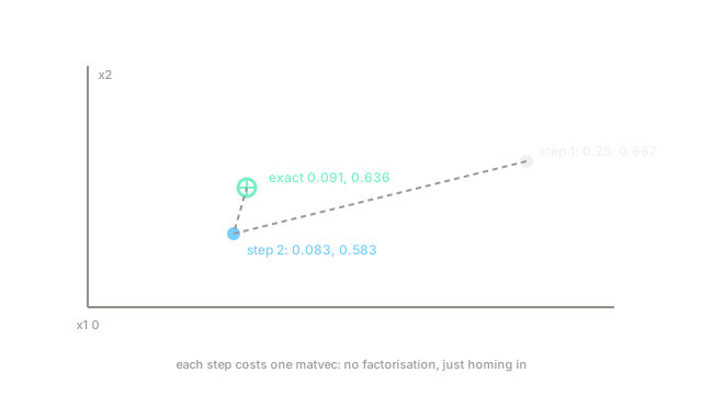
Solve $\begin{bmatrix} 4 & 1 \\ 1 & 3 \end{bmatrix} x = \begin{bmatrix} 1 \\ 2 \end{bmatrix}$ by Jacobi from $x_0 = [0, 0]$ . The exact answer is $[1/11, 7/11] \approx [0.0909, 0.6364]$ .

Step 1: $x_1 = [1/4, 2/3] = [0.25, 0.6667]$
Step 2: $x_2 = [(1 - 0.6667)/4, (2 - 0.25)/3] = [0.0833, 0.5833]$

Two cheap steps land at $[0.0833, 0.5833]$ , already within $0.06$ of $[0.0909, 0.6364]$ . Diagonal dominance ( $4 > 1$ , $3 > 1$ ) guarantees the march continues to the answer. Gauss-Seidel would reuse $0.25$ inside step 1's second coordinate and arrive slightly faster.

Code

The point is the check: run Jacobi and confirm the iterates approach the exact answer.

1def jacobi(a11: float, a12: float, a21: float, a22: float, b1: float, b2: float, steps: int) -> list[float]:2    x1, x2 = 0.0, 0.03    for _ in range(steps):4        x1, x2 = (b1 - a12 * x2) / a11, (b2 - a21 * x1) / a225    return [x1, x2]6
7
8print([round(v, 4) for v in jacobi(4, 1, 1, 3, 1, 2, 1)])  # -> [0.25, 0.6667]9print([round(v, 4) for v in jacobi(4, 1, 1, 3, 1, 2, 2)])  # -> [0.0833, 0.5833]

Note the subtlety the code hides: both updates in one line use the old pair on the right (tuple assignment evaluates first), which is exactly Jacobi semantics. Gauss-Seidel would assign sequentially instead.

Watch Out For

Running conjugate gradient on a non-SPD matrix

CG minimises an energy that exists only for symmetric positive definite $A$ . On indefinite or asymmetric systems it can stagnate, oscillate or return confident garbage with a small residual in the wrong norm. Verify SPD (Cholesky succeeds, eigenvalues positive) before CG; otherwise reach for GMRES or MINRES, which handle asymmetry and indefiniteness respectively.

Iterating an ill-conditioned system without a preconditioner

CG converges in $O(\sqrt{\kappa})$ steps, so $\kappa = 10^6$ means a thousand iterations of expensive matvecs. A preconditioner $M \approx A$ that is cheap to invert clusters the spectrum of $M^{-1}A$ and collapses the count. Jacobi itself doubles as the cheapest preconditioner (diagonal scaling). Unpreconditioned iteration on hard problems is how clusters burn budgets.

The Quick Version

Iterative solvers refine guesses per matvec instead of factoring at $O(n^3)$ .
Jacobi updates from stale values; Gauss-Seidel reuses fresh ones; CG finishes SPD systems via conjugate directions.
Two Jacobi steps reach $[0.0833, 0.5833]$ , near the exact $[0.0909, 0.6364]$ .
Convergence needs conditions: diagonal dominance, or SPD for CG.
CG on non-SPD input and unpreconditioned runs on ill-conditioned systems are the two classic failures.