Sparse Matrix Methods

Store only the nonzeros, compute only on nonzeros. Real matrices are mostly empty, and the format you pick decides whether code flies or crawls.

A path graph Laplacian is nearly all empty with nonzeros only on three diagonals, so CSR stores 3n values instead of n squared and matvec touches only those

Why Does This Exist?

Dense storage of a $10^6 \times 10^6$ matrix needs $10^{12}$ numbers: eight terabytes in doubles. But real giant matrices are mostly zero. A path graph's Laplacian holds $3n - 2$ nonzeros out of $n^2$ entries. A document-term matrix is 99.9% empty. Finite-element meshes touch only neighbours. Sparse methods store the nonzeros plus their addresses, and every operation (matvec, factorisation, eigensolve) runs on that compressed form. Without them, giant+sparse problems simply do not fit.

The catch is structure. Sparsity patterns decide everything: which format streams fastest, whether factorisation stays sparse (fill-in) or densifies catastrophically, and which iterative solver converges. Dense habits (toarray(), direct factoring, random access) applied to sparse giants are the standard way to OOM a cluster.

The one idea you need first

Nnz counts stored nonzeros. A sparse matvec costs $O(\text{nnz})$ , not $O(n^2)$ : each nonzero multiplies once. Formats differ in how they index those nonzeros: COO lists triples, CSR compresses row pointers for row streaming, CSC mirrors it for columns. Pick by access pattern.

Think of It Like This

A library that shelves only borrowed books

A library with a million catalogue entries but only three thousand books ever borrowed could shelve all million slots (dense: room-sized, mostly empty shelves) or keep the borrowed three thousand plus a card index of where each belongs (sparse: one wall plus the index).

Browsing by shelf order (row access) wants the cards sorted by shelf: CSR. Browsing by author across shelves (column access) wants the transposed index: CSC. Reorganising the whole library (factorisation) pulls new books "into use" as shelves shift: fill-in, the phenomenon that turns sparse factors dense unless the ordering (AMD, nested dissection) controls it.

How It Actually Works

The working set:

COO: (row, col, value) triples. Build incrementally, then convert; never compute in it.
CSR: values plus column indices plus row-start pointers. Row slicing and matvec stream; column writes crawl. The default workhorse.
CSC: the transpose layout. Column slicing, and the format most sparse direct solvers factor in.
Fill-in: factoring creates nonzeros where $A$ had zeros (a nonzero path $i \to k \to j$ fills $(i,j)$ during elimination). Reorder first (approximate minimum degree, nested dissection) to starve those paths.
Solvers: Krylov iterations (iterative solvers) with incomplete-factorisation or multigrid preconditioners; Lanczos/LOBPCG for extremal eigenpairs.

Worked example

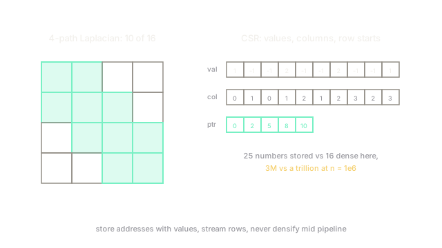
The 4-node path graph $1-2-3-4$ has Laplacian:

L = \begin{bmatrix} 1 & -1 & 0 & 0 \\ -1 & 2 & -1 & 0 \\ 0 & -1 & 2 & -1 \\ 0 & 0 & -1 & 1 \end{bmatrix}

Nonzeros: $4$ diagonal plus $6$ off-diagonal $= 10$ of $16$ entries. CSR stores $10$ values, $10$ column indices and $5$ row pointers: $25$ numbers against $16$ dense, barely a win at $n = 4$ . Scale to a million-node path: $3 \times 10^6 - 2$ nonzeros against $10^{12}$ dense entries, a factor of $300{,}000$ in memory. That ratio is why/traffic networks, meshes and graphs live sparse-only, and why one accidental densification ends the job.

Code

The point is the check: multiply sparsely with a dictionary-of-rows and confirm against the dense answer.

1def sparse_matvec(rows: dict[int, dict[int, float]], x: list[float]) -> list[float]:2    n = len(x)3    out = [0.0] * n4    for i, cols in rows.items():  # touch stored entries only5        out[i] = sum(v * x[j] for j, v in cols.items())6    return out7
8
9L = {0: {0: 1.0, 1: -1.0}, 1: {0: -1.0, 1: 2.0, 2: -1.0},10     2: {1: -1.0, 2: 2.0, 3: -1.0}, 3: {2: -1.0, 3: 1.0}}11print(sparse_matvec(L, [1.0, 2.0, 3.0, 4.0]))  # -> [-1.0, 0.0, 0.0, 1.0]

Check row one: $-1 + 4 - 3 = 0$ ✓. Ten multiply-adds instead of sixteen, and the ratio improves without bound as $n$ grows.

Watch Out For

Densifying a sparse matrix mid-pipeline

One .toarray(), one dense identity added, one careless + with a dense matrix, and the $3 \times 10^6$ nonzeros become $10^{12}$ dense entries: instant OOM on hardware that held the sparse form at 1%. Audit every operation's output format, and treat densification calls as seriously as unguarded recursion.

Factoring sparse without reordering

Sparse LU without a fill-reducing ordering can densify factors until they exceed dense storage: the mesh that stored in megabytes factors into gigabytes. Always reorder (AMD or nested dissection come free in every sparse solver) before factoring, and prefer iterative-plus-preconditioner when factors threaten to fill.

The Quick Version

Sparse methods store nonzeros plus addresses; matvec costs $O(\text{nnz})$ , never $O(n^2)$ .
CSR streams rows, CSC streams columns, COO builds: pick by access pattern.
The 4-path Laplacian holds 10 of 16; the million-path holds 3M of a trillion.
Factorisation creates fill-in: reorder first or go iterative with a preconditioner.
One accidental densification OOMs what sparsity made possible: audit output formats.