Sub-Gaussian and Sub-Exponential Variables

Two ways to say a random variable has a thin tail. Sub-Gaussian tails vanish like a Gaussian, sub-exponential tails vanish a little slower, and both give you exponential concentration for averages.

A Gaussian-like tail drops steeply while an exponential tail drops more slowly, and both sit far below the Chebyshev curve past two units

Why Does This Exist?

Averages are the workhorse of learning: training loss, validation error and gradient estimates are all means. Markov and Chebyshev inequalities bound those means with only a variance, but the bound decays like $1/t^2$ , which is painfully slow. To promise that 1,000 samples pin a mean within $0.1$ , you want a bound that decays like $\exp(-ct^2)$ , exponentially fast.

Sub-Gaussian and sub-exponential variables are the two classes where that fast decay holds. Bounded variables like coin flips, Gaussians themselves and averages of many small independent effects all qualify. This page defines both classes, shows the tail each one buys, and gives the one worked number you will reuse everywhere. Concentration of measure then applies the same idea to functions, and high-dimensional probability and statistics shows why it matters when dimensions pile up.

Prerequisite in one paragraph. You need the moment generating function $M(\lambda) = E[\exp(\lambda X)]$ , which is the expected value of the exponential of $\lambda X$ ; it encodes all moments at once. If $X$ has mean zero, $M(0) = 1$ and the growth of $M$ controls the tails. Background on means and spreads is in expectation, variance and covariance.

Think of It Like This

Two kinds of leash on a dog

A sub-Gaussian dog wears a short elastic leash. The further it runs, the harder the leash pulls back, quadratically. It almost never gets far. A sub-exponential dog wears a longer rope leash. Near you it behaves the same, but once it builds speed the restraint is only linear, so rare long runs happen more often.

Both dogs stay close almost all the time, which is what concentration needs. But if you plan a fence from the Gaussian formula while walking the rope-leash dog, the rare escape surprises you. Knowing which leash you hold decides which bound you may quote.

Where the analogy stops: real tails are about chance, not force. The leash never physically pulls; it just says far outcomes are rare in a precise quantitative way.

How It Actually Works

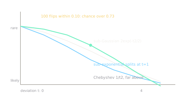
A mean-zero variable $X$ is sub-Gaussian with variance proxy $\sigma^2$ (a number playing the role of variance in the bound) when its moment generating function satisfies $E[\exp(\lambda X)] \le \exp(\sigma^2 \lambda^2 / 2)$ for every real $\lambda$ . In words: the exponential moments grow no faster than a Gaussian with variance $\sigma^2$ . The payoff is the tail bound $P(|X| \ge t) \le 2\exp(-t^2 / 2\sigma^2)$ , where $P$ is chance and $t$ is the deviation size.

A mean-zero $X$ is sub-exponential with parameters $(\nu, b)$ when $E[\exp(\lambda X)] \le \exp(\nu^2\lambda^2/2)$ for $|\lambda| < 1/b$ . Same shape near zero, but the control stops at $1/b$ . The tail splits: $P(|X| \ge t) \le 2\exp(-t^2/2\nu^2)$ for small $t$ (Gaussian-like centre) and $2\exp(-t/2b)$ for large $t$ (exponential far tail). Squares of Gaussians and exponential variables live here.

The two facts you will quote weekly: any variable bounded in $[a, b]$ is sub-Gaussian with $\sigma^2 = (b-a)^2/4$ , and a sum of $n$ independent sub-Gaussians with proxy $\sigma^2$ is sub-Gaussian with proxy $n\sigma^2$ , so its average has proxy $\sigma^2/n$ . Averages inherit thin tails with the proxy shrinking like $1/n$ .

Worked example

Flip a fair coin 100 times and track the fraction of heads $\bar{X}$ . Each flip shifted to mean zero lives in $[-0.5, 0.5]$ , so each is sub-Gaussian with $\sigma^2 = (1)^2/4 = 0.25$ . The average over 100 flips has proxy $0.25/100 = 0.0025$ , meaning $\sigma = 0.05$ .

Ask for deviation $t = 0.10$ , that is, the fraction leaving $[0.40, 0.60]$ . The bound gives $P(|\bar{X} - 0.5| \ge 0.10) \le 2\exp(-0.10^2 / (2 \times 0.0025)) = 2\exp(-0.01/0.005) = 2\exp(-2) \approx 2 \times 0.1353 = 0.2706$ . So chance above $0.73$ of staying inside. Tighten with Hoeffding's exact constant for bounded sums, $2\exp(-2nt^2) = 2\exp(-2 \times 100 \times 0.01) = 2\exp(-2) \approx 0.27$ , same number. Chebyshev would only give variance $0.0025$ over $0.01$ , a useless bound of $0.25$ on the nose with no exponential improvement as $n$ grows.

Watch Out For

Quoting a Gaussian tail for a squared Gaussian

If $Z$ is standard normal, $Z$ is sub-Gaussian but $Z^2 - 1$ is only sub-exponential. Its far tail decays like $\exp(-ct)$ , not $\exp(-ct^2)$ . Plugging the Gaussian formula underestimates the chance of a large chi-squared deviation by orders of magnitude, which is exactly how a variance estimate blows past its supposed confidence band.

Fix: squares, products and norms of sub-Gaussians are sub-exponential. Switch to the Bernstein split tail the moment a square appears.

Treating the variance proxy as the variance

The proxy $\sigma^2$ is an upper control, not the actual variance. A Rademacher flip taking values $\pm 1$ has variance $1$ and smallest valid proxy $1$ , fine. But a bounded variable in $[0, 1]$ with tiny true variance still gets proxy $0.25$ from the interval length. Using $0.25$ where the true variance is $0.01$ loosens every downstream sample-size calculation by a factor of 25.

Fix: the proxy is safe but pessimistic. When the true variance is much smaller than the range suggests, reach for Bernstein, which uses both.

The Quick Version

Sub-Gaussian means exponential moments grow at most like a Gaussian, giving tail $2\exp(-t^2/2\sigma^2)$ .
Sub-exponential matches that near zero but switches to $2\exp(-t/2b)$ far out.
Anything bounded in $[a,b]$ is sub-Gaussian with proxy $(b-a)^2/4$ .
Averages of $n$ independent sub-Gaussians shrink the proxy by $1/n$ , so 100 flips stay within 0.10 of half with chance above 0.73.
Squares of sub-Gaussians are sub-exponential, never sub-Gaussian.