Degrees of Freedom and Robot Bodies

Why Does This Exist?

When commanding a robotic manipulator or mobile rover, you want to tell it where to place its tool or where to drive on the floor. But you cannot simply command arbitrary spatial targets: a robot cannot reach a point further than the sum of its limbs, cannot slide sideways if its wheels are locked forward, and cannot rotate its wrist through its own mechanical base.

Degrees of Freedom (DoF) provide the fundamental accounting system for robotic mechanics. They tell you:

1. How many independent numbers are required to define the robot's complete posture.
2. What physical volume of space the robot can actually reach (its workspace).
3. Whether the robot has redundancy to maneuver around obstacles while holding a tool fixed.

Without this accounting, planners request impossible poses, policies command motions into self-collisions, and algorithms confuse joint space with task space.

Basics first: the electromechanical motors driving each degree of freedom live in robot-anatomy. How coordinates transform between the robot base and hand lives in robot-coordinate-frames. Solving for the exact joint angles that place the hand at a target lives in robot-forward-inverse-kinematics.

Think of It Like This

How It Actually Works

Configuration space ($\mathcal{C}$-space) versus Task space

To control a robot, we must distinguish between two different mathematical spaces:

• Configuration Space ($\mathcal{C}$-space): The space of all possible joint states. For an $n$-joint serial arm with revolute joints, a single configuration is a vector of angles $\mathbf{q} = (\theta_1, \theta_2, \ldots, \theta_n) \in \mathcal{C}$. The dimension of $\mathcal{C}$-space is exactly $n$.
• Task Space (Operational Space): The space where the robot's physical task is specified, typically rigid-body poses in $SE(3)$ (dimension 6: $x, y, z$ position and roll, pitch, yaw orientation) or planar poses in $SE(2)$ (dimension 3: $x, y, \theta$).

When $n < 6$, the arm is underactuated for full 3D manipulation: it cannot achieve arbitrary poses. When $n = 6$, there is typically a finite set of discrete configurations that reach a given target pose. When $n > 6$, the arm is kinematically redundant: an infinite continuous manifold of arm postures can hold the exact same end-effector pose.

Holonomic versus nonholonomic systems

Having $n$ degrees of freedom in configuration does not mean you have $n$ independent velocity controls at any instant:

• Holonomic robots: Can instantly accelerate along all configuration coordinates. An omnidirectional mobile base with Mecanum wheels can translate sideways, drive forward, or spin in place instantaneously ($3$ controllable velocity DoF in $SE(2)$).
• Nonholonomic robots: Suffer from differential motion constraints. A standard differential-drive mobile base or car has a 3D configuration $(x, y, \theta)$, but only 2 control inputs (forward speed $v$ and turn rate $\omega$). It cannot slide sideways instantaneously ($\dot{y}\cos\theta - \dot{x}\sin\theta = 0$). Parallel parking requires maneuvering forward and backward because lateral velocity is constrained to zero.

Worked example: workspace of a 2-link planar arm

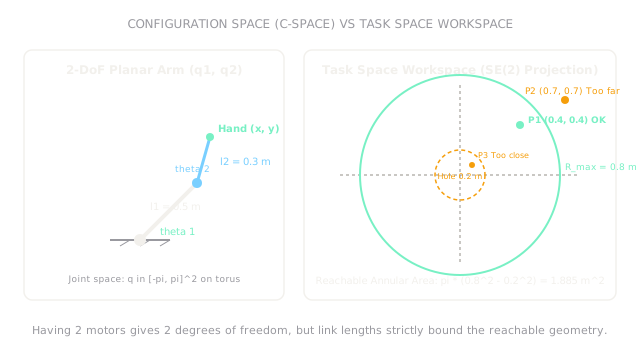
Consider a planar arm moving in the $xy$-plane with two revolute joints and rigid links of lengths $l_1 = 0.5\text{ m}$ and $l_2 = 0.3\text{ m}$.

• Joint space: $\mathbf{q} = (\theta_1, \theta_2) \in [-\pi, \pi) \times [-\pi, \pi) = \mathbb{T}^2$ (a 2D torus).
• Task space: Target end-effector coordinates $(x, y) \in \mathbb{R}^2$.

The maximum reach occurs when the arm is fully extended ($\theta_2 = 0$):

The minimum reach occurs when the second link folds fully back along the first link ($\theta_2 = \pi$):

The reachable workspace is an annulus (ring) centered at the base origin $(0, 0)$. Its surface area $A$ is:

Now evaluate reachability for three candidate target points:

1. Target $P_1 = (0.4, 0.4)\text{ m}$: $d_1 = \sqrt{0.4^2 + 0.4^2} = \sqrt{0.16 + 0.16} = \sqrt{0.32} \approx 0.566\text{ m}$ Since $0.2 \le 0.566 \le 0.8$, target $P_1$ is reachable inside the annular workspace.
2. Target $P_2 = (0.7, 0.7)\text{ m}$: $d_2 = \sqrt{0.7^2 + 0.7^2} = \sqrt{0.49 + 0.49} = \sqrt{0.98} \approx 0.990\text{ m}$ Since $0.990 > 0.8$, target $P_2$ is unreachable (lies beyond maximum reach).
3. Target $P_3 = (0.1, 0.1)\text{ m}$: $d_3 = \sqrt{0.1^2 + 0.1^2} = \sqrt{0.01 + 0.01} = \sqrt{0.02} \approx 0.141\text{ m}$ Since $0.141 < 0.2$, target $P_3$ is unreachable (lies inside the central inner singularity hole).

Code

This Python snippet defines the 2-link arm kinematics boundaries, computes the workspace area, and tests candidate Cartesian targets for geometric reachability.

1import math2
3
4def check_planar_reachability(5    l1: float,6    l2: float,7    points: list[tuple[float, float]],8) -> tuple[float, float, float, list[bool]]:9    """Compute workspace limits, annular area, and evaluate reachability of points."""10    r_max: float = l1 + l211    r_min: float = abs(l1 - l2)12    area: float = math.pi * (r_max ** 2 - r_min ** 2)13
14    reachability: list[bool] = []15    for x, y in points:16        dist: float = math.hypot(x, y)17        reachability.append(r_min <= dist <= r_max)18
19    return round(r_max, 3), round(r_min, 3), round(area, 3), reachability20
21
22r_max, r_min, area, results = check_planar_reachability(23    l1=0.5,24    l2=0.3,25    points=[(0.4, 0.4), (0.7, 0.7), (0.1, 0.1)],26)27
28print(r_max)    # -> 0.829print(r_min)    # -> 0.230print(area)     # -> 1.88531print(results)  # -> [True, False, False]

Watch Out For

The Quick Version

• Degrees of freedom (DoF) represent the minimum number of independent coordinates needed to uniquely describe a robot's physical configuration.
• Configuration space ($\mathcal{C}$-space) has dimension equal to the number of joints, whereas task space is the 3D ($SE(3)$) or planar ($SE(2)$) environment.
• A 2-link planar arm ($l_1=0.5\text{ m}, l_2=0.3\text{ m}$) sweeps an annular workspace with outer radius $0.8\text{ m}$ and inner unreachable hole $0.2\text{ m}$, enclosing $1.885\text{ m}^2$.
• Holonomic systems can accelerate along all coordinates instantaneously; nonholonomic systems (like cars and differential rovers) have velocity constraints that prohibit sideways sliding.
• Redundant manipulators ($> 6\text{ DoF}$) can reconfigure internal joint postures (elbow angles) while holding the end-effector perfectly still.

What to Read Next

• Robot Anatomy: Sensors, Actuators and Compute
• Coordinate Frames and Transformations
• Forward and Inverse Kinematics
• Robot Motion Planning