Forward and Inverse Kinematics

Why Does This Exist?

When commanding a robotic arm, the goal is expressed in operational task coordinates: "place the suction gripper at coordinate $(x=0.6, y=0.4)$ on the conveyor belt." But motors do not accept Cartesian $(x, y)$ coordinates. Motors rotate joints through individual angles $(\theta_1, \theta_2, \ldots, \theta_n)$.

Mapping between these two representations is the domain of kinematics:

• Forward Kinematics (FK): Given joint angles $\mathbf{q}$, where is the hand? This is a forward geometric evaluation: every joint angle yields exactly one unique end-effector pose.
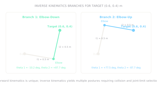
• Inverse Kinematics (IK): Given a desired hand pose $\mathbf{x}$, what joint angles $\mathbf{q}$ reach it? This is fundamentally difficult: non-linear trigonometric equations yield multiple solution branches (e.g. elbow-up versus elbow-down), boundary singularities where joints lock up, or no solution if the target lies outside the arm's reach.

Solving inverse kinematics reliably is the bridge that allows high-level trajectory planners to command low-level joint motor drives.

Basics first: the configuration space and workspace geometry of robotic limbs live in robot-degrees-of-freedom. Transforming between base and tool frames lives in robot-coordinate-frames. Generating collision-free paths between joint configurations lives in robot-motion-planning.

Think of It Like This

How It Actually Works

The 2-link planar arm forward kinematics

For a planar 2-link arm with link lengths $l_1$ and $l_2$, and joint angles $\theta_1$ and $\theta_2$, the end-effector position $(x, y)$ is given by simple trigonometry:

This forward mapping is unique, continuous, and straightforward to evaluate.

Inverse kinematics via the Law of Cosines

Given a target position $(x, y)$, we first compute the squared distance from the base origin:

If $r > l_1 + l_2$ or $r < |l_1 - l_2|$, the target is outside the reachable workspace and no physical solution exists.

Inside the workspace, applying the Law of Cosines to the triangle formed by $l_1$, $l_2$, and $r$ gives:

Solving for $\cos(\theta_2)$:

Because $\cos(\theta_2) = \cos(-\theta_2)$, there are two distinct solutions for joint 2:

Once $\theta_2$ is selected, $\theta_1$ is found by projecting angles:

• $\theta_2 > 0$ corresponds to the elbow-down configuration.
• $\theta_2 < 0$ corresponds to the elbow-up configuration.

Kinematic singularities: losing degrees of freedom

A singularity occurs when the arm loses the ability to move in one or more Cartesian directions. For the 2-link arm, this happens when:

• $\theta_2 = 0$: The arm is fully outstretched ($r = l_1 + l_2$). The arm cannot produce radial velocity outward.
• $\theta_2 = \pi$: The arm is folded completely onto itself ($r = |l_1 - l_2|$).

At a singularity, the Jacobian matrix drops rank. Attempting to track a Cartesian path through a singularity demands mathematically infinite joint velocities ($\dot{\mathbf{q}} = \mathbf{J}^{-1} \dot{\mathbf{x}}$), causing motor drives to trip overcurrent or velocity safety limits.

Worked example: solving IK for target $(0.6, 0.4)\text{ m}$

Consider a 2-link arm with equal link lengths $l_1 = 0.5\text{ m}$ and $l_2 = 0.5\text{ m}$. We want to reach target $(x, y) = (0.6, 0.4)\text{ m}$.

Compute squared distance $r^2$:

Distance $r = \sqrt{0.52} \approx 0.7211\text{ m}$. Since $0.0 \le 0.7211 \le 1.0\text{ m}$, the target is reachable.

Compute $\cos(\theta_2)$:

Compute the two joint 2 branches:

Compute base angle $\beta = \text{atan2}(y, x)$:

For Branch 1 (Elbow-Down, $\theta_2 = +1.5308\text{ rad}$):

For Branch 2 (Elbow-Up, $\theta_2 = -1.5308\text{ rad}$):

Forward kinematics confirms both branches reach $(0.6, 0.4)\text{ m}$ exactly:

• Elbow-down: $\theta_1 = -10.16^\circ, \theta_2 = +87.71^\circ \implies (0.60, 0.40)\text{ m}$.
• Elbow-up: $\theta_1 = +77.54^\circ, \theta_2 = -87.71^\circ \implies (0.60, 0.40)\text{ m}$.

Code

This Python snippet implements forward and inverse kinematics for the 2-link planar arm, verifies both solution branches, and tests for singularity boundary detection.

1import math2
3
4def solve_2link_ik(5    l1: float,6    l2: float,7    x: float,8    y: float,9) -> tuple[tuple[float, float], tuple[float, float]] | None:10    """Solve inverse kinematics for 2-link planar arm returning (elbow_down, elbow_up) in degrees."""11    r2: float = x ** 2 + y ** 212    cos_th2: float = (r2 - l1 ** 2 - l2 ** 2) / (2.0 * l1 * l2)13
14    if abs(cos_th2) > 1.0:15        return None  # Target unreachable16
17    th2_down: float = math.acos(cos_th2)18    th2_up: float = -th2_down19
20    beta: float = math.atan2(y, x)21    psi: float = math.atan2(l2 * math.sin(th2_down), l1 + l2 * math.cos(th2_down))22
23    th1_down: float = beta - psi24    th1_up: float = beta + psi25
26    return (27        (round(math.degrees(th1_down), 2), round(math.degrees(th2_down), 2)),28        (round(math.degrees(th1_up), 2), round(math.degrees(th2_up), 2)),29    )30
31
32solutions = solve_2link_ik(l1=0.5, l2=0.5, x=0.6, y=0.4)33if solutions is not None:34    elbow_down, elbow_up = solutions35    print(elbow_down)  # -> (-10.16, 87.71)36    print(elbow_up)    # -> (77.54, -87.71)

Watch Out For

The Quick Version

• Forward kinematics uniquely maps joint coordinates $\mathbf{q}$ to end-effector pose $(x, y, z)$ using geometric link transformations.
• Inverse kinematics recovers joint angles from a desired Cartesian target; it is non-linear and produces multiple solution branches.
• For a 2-link planar arm ($l_1=l_2=0.5\text{ m}$) reaching $(0.6, 0.4)\text{ m}$, the Law of Cosines yields two branches: elbow-down $(-10.16^\circ, +87.71^\circ)$ and elbow-up $(+77.54^\circ, -87.71^\circ)$.
• Singularity configurations occur at workspace boundaries (full extension or folding), where the arm loses an instantaneous degree of freedom.
• Continuous trajectory tracking must maintain configuration branch consistency to prevent catastrophic joint flips during motion.

What to Read Next

• Degrees of Freedom and Robot Bodies
• Coordinate Frames and Transformations
• Robot Motion Planning
• Feedback Control and PID