Robot Motion Planning

Motion planning finds a collision-free geometric path from start to goal in the robot's configuration space, then parameterizes it into a dynamically feasible trajectory that respects velocity, acceleration, and jerk limits.

Motion planning expands obstacles by robot radius to navigate configuration space, timing paths into feasible trajectories

Why Does This Exist?

If you treat a robot as an infinitesimal point, finding a route between two coordinates is a straightforward 2D maze search. But real physical robots have volume: a delivery rover has a 50-centimeter chassis with protruding wheels, and a 6-axis manipulator has thick aluminum links that sweep a broad 3D volume as they articulate.

If a path planner routes an arm right along the edge of a shelf, the fingertip might clear the edge while the elbow punches straight through the wood. Furthermore, even if a geometric line of waypoints is collision-free, a physical robot cannot instantly change direction: electric motors have finite torque, leading to maximum acceleration and jerk boundaries.

Motion planning bridges this gap through two critical abstractions:

Configuration space ( $\mathcal{C}$ -space) obstacles: By growing physical obstacles by the robot's physical geometry (via Minkowski sums), the robot is shrunk to a single mathematical point, converting complex volumetric collision queries into simple point containment tests.
Trajectory parameterization: Parameterizing a static geometric path into a time-indexed trajectory $\mathbf{q}(t)$ with smooth velocity profiles that motor controllers can physically track.

Basics first: the joint coordinates that define configuration space live in robot-degrees-of-freedom. Converting operational poses to joint waypoints lives in robot-forward-inverse-kinematics. Re-planning trajectories online against dynamic obstacles lives in robot-model-predictive-control.

Think of It Like This

Navigating a wide furniture dolly through a narrow doorway

Imagine pushing a heavy, wide wooden wardrobe on a four-wheeled dolly through an apartment doorway.

You do not simply aim for the open space between the door frames. You look at the width of the wardrobe and mentally "fatten" the door frame inwards on both sides by half the wardrobe's width. In your mind, the wide doorway shrinks to a narrow passage. If the center of your dolly can pass through that shrunken gap, you know the physical edges of the wardrobe will not scrape the paint off the door jambs.

Where it stops: a human mover can pause, tilt the wardrobe at a $45^\circ$ angle, or squeeze through foam padding. In high-dimensional robotics (such as a 7-axis arm moving through a cluttered engine bay), $\mathcal{C}$ -space obstacles are complex non-linear manifolds that cannot be visualized directly, requiring sampling algorithms (like RRT or PRM) to explore the free space.

How It Actually Works

The Minkowski sum and $\mathcal{C}$ -space obstacles

Let the robot body be a rigid set of points $\mathcal{A} \subset \mathbb{R}^d$ , and let obstacles in the workspace be $\mathcal{B} \subset \mathbb{R}^d$ . When the robot is located at configuration $\mathbf{q}$ , its physical footprint is $\mathcal{A}(\mathbf{q})$ .

The configuration space obstacle region $\mathcal{C}_{\text{obs}}$ is the set of all configurations where the robot intersects an obstacle:

\mathcal{C}_{\text{obs}} = \{\mathbf{q} \in \mathcal{C} \mid \mathcal{A}(\mathbf{q}) \cap \mathcal{B} \ne \emptyset\}

For a circular robot of radius $R_{\text{robot}}$ translating in 2D space, the $\mathcal{C}$ -space obstacle for a circular obstacle of radius $r_{\text{obs}}$ is computed via the Minkowski sum:

R_{\mathcal{C}} = r_{\text{obs}} + R_{\text{robot}}

In $\mathcal{C}$ -space, the robot is represented as a single point at $(x, y)$ , and the obstacle is enlarged to radius $R_{\mathcal{C}}$ . A point path is collision-free if and only if it never enters any expanded $\mathcal{C}_{\text{obs}}$ circle.

Graph search versus sampling-based planning

Grid / Graph Search (A*, Dijkstra): Discretizes $\mathcal{C}$ -space into an explicit grid. Guarantees finding the optimal path if one exists (resolution completeness), but scales exponentially $\mathcal{O}(k^d)$ with configuration dimension $d$ . Effective for 2D mobile bases, intractable for 7-DoF arms.
Sampling-Based Planners (RRT, PRM): Explores continuous high-dimensional $\mathcal{C}$ -space by generating random configuration samples $\mathbf{q}_{\text{rand}}$ , steering toward them, and checking collision along the local edge. Rapidly-exploring Random Trees (RRT) bias growth toward unexplored Voronoi regions, finding feasible paths in high dimensions within milliseconds (probabilistically complete).

From geometric path to timed trajectory

A geometric path $\sigma(s)$ specifies positions parameterized by distance $s \in [0, L]$ . A trajectory $\mathbf{q}(t)$ assigns time to every point, establishing velocities $\dot{\mathbf{q}}(t)$ and accelerations $\ddot{\mathbf{q}}(t)$ .

A standard industrial trajectory profile is the trapezoidal velocity profile:

Phase 1 (Acceleration): Accelerate at $+a_{\max}$ until reaching cruise speed $v_{\max}$ .
Phase 2 (Cruise): Cruise at constant velocity $v_{\max}$ .
Phase 3 (Deceleration): Decelerate at $-a_{\max}$ to stop smoothly at the goal.

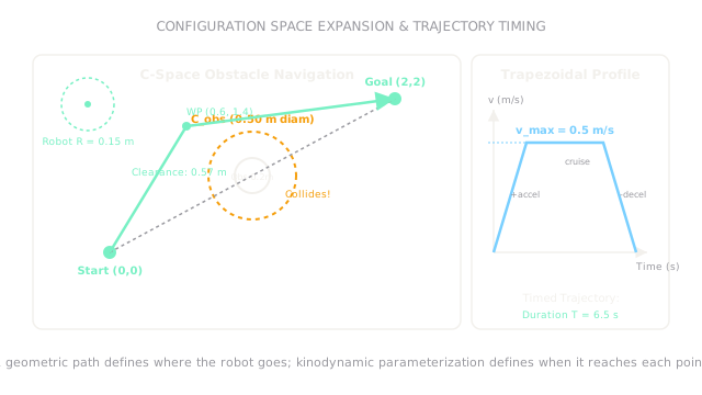
Worked example: navigating an obstacle and trajectory timing

A circular mobile robot navigates an indoor floor:

Robot radius: $R_{\text{robot}} = 0.15\text{ m}$ ( $15\text{ cm}$ ).
Circular pillar obstacle centered at $(x_o, y_o) = (1.0, 1.0)\text{ m}$ with physical diameter $0.20\text{ m}$ ( $r_{\text{obs}} = 0.10\text{ m}$ ).
Start: $(0.0, 0.0)\text{ m}$ , Goal: $(2.0, 2.0)\text{ m}$ .

First, compute the $\mathcal{C}$ -space obstacle radius and diameter:

R_{\mathcal{C}} = r_{\text{obs}} + R_{\text{robot}} = 0.10 + 0.15 = 0.25\text{ m} \implies \text{Diameter} = 0.50\text{ m}

A direct straight-line path from $(0,0)$ to $(2,2)$ passes through $(1.0, 1.0)$ , penetrating $0.25\text{ m}$ into $\mathcal{C}_{\text{obs}}$ (unavoidable collision).

The planner introduces an intermediate waypoint $W = (0.60, 1.40)\text{ m}$ . Check clearance from waypoint to obstacle center:

d = \sqrt{(0.60 - 1.0)^2 + (1.40 - 1.0)^2} = \sqrt{(-0.4)^2 + 0.4^2} = \sqrt{0.16 + 0.16} = \sqrt{0.32} \approx 0.566\text{ m}

Clearance margin beyond the $\mathcal{C}$ -space obstacle:

\text{Margin} = d - R_{\mathcal{C}} = 0.566 - 0.250 = 0.316\text{ m} = 31.6\text{ cm} \quad (\text{Safe!})

Now compute total path length $L$ :

L_1 = \sqrt{0.6^2 + 1.4^2} = \sqrt{0.36 + 1.96} = \sqrt{2.32} \approx 1.523\text{ m}

L_2 = \sqrt{(2.0 - 0.6)^2 + (2.0 - 1.4)^2} = \sqrt{1.4^2 + 0.6^2} = \sqrt{2.32} \approx 1.523\text{ m}

L_{\text{total}} = 1.523 + 1.523 = 3.046\text{ m}

Time parameterization with $v_{\max} = 0.50\text{ m/s}$ and $a_{\max} = 0.50\text{ m/s}^2$ :

Acceleration time: $t_a = v_{\max} / a_{\max} = 0.50 / 0.50 = 1.0\text{ s}$ .
Distance traveled during acceleration: $d_a = \frac{1}{2} a t_a^2 = 0.5(0.5)(1.0) = 0.25\text{ m}$ .
Deceleration distance: $d_d = 0.25\text{ m}$ ( $t_d = 1.0\text{ s}$ ).
Cruise distance: $d_{\text{cruise}} = 3.046 - (0.25 + 0.25) = 2.546\text{ m}$ .
Cruise time: $t_{\text{cruise}} = 2.546 / 0.50 = 5.092\text{ s}$ .
Total trajectory duration: $T = 1.0 + 5.092 + 1.0 \approx 7.09\text{ s}$ (smooth, bounded jerk and acceleration).

Code

This Python snippet defines the $\mathcal{C}$ -space obstacle expansion, tests waypoint clearance, and generates the time-parameterized trapezoidal velocity profile.

1import math2
3
4def plan_timed_path(5    r_robot: float,6    r_obs: float,7    obs_center: tuple[float, float],8    waypoint: tuple[float, float],9    v_max: float = 0.50,10    a_max: float = 0.50,11) -> tuple[float, float, bool, float]:12    """Compute C-space obstacle radius, clearance, safety check, and total duration."""13    r_cspace: float = r_robot + r_obs14    dist_to_obs: float = math.hypot(15        waypoint[0] - obs_center[0],16        waypoint[1] - obs_center[1],17    )18    is_safe: bool = dist_to_obs > r_cspace19
20    # 2-segment path: (0,0) -> WP -> (2,2)21    l1: float = math.hypot(waypoint[0], waypoint[1])22    l2: float = math.hypot(2.0 - waypoint[0], 2.0 - waypoint[1])23    total_len: float = l1 + l224
25    # Trapezoidal profile timing26    t_accel: float = v_max / a_max27    d_accel: float = 0.5 * a_max * (t_accel ** 2)28    d_cruise: float = total_len - 2.0 * d_accel29    t_cruise: float = d_cruise / v_max30    total_time: float = 2.0 * t_accel + t_cruise31
32    return round(r_cspace, 3), round(dist_to_obs, 3), is_safe, round(total_time, 2)33
34
35r_c, clearance, safe, duration = plan_timed_path(36    r_robot=0.15,37    r_obs=0.10,38    obs_center=(1.0, 1.0),39    waypoint=(0.6, 1.4),40)41
42print(r_c)        # -> 0.2543print(clearance)  # -> 0.56644print(safe)       # -> True45print(duration)   # -> 7.09

Watch Out For

Assuming a geometric path can be executed at maximum speed

A path is merely an ordered set of geometric waypoints without timestamps. If an execution script commands motor drives to hit each waypoint at maximum velocity without accounting for cornering acceleration, the motors demand infinite acceleration at sharp turns.

The symptom is severe trajectory tracking error, cutting corners, or tripping overcurrent faults. Fix it by passing geometric paths through a kinodynamic trajectory smoother (such as Time-Optimal Path Parameterization, TOPP-RA, or cubic splines) that enforces joint velocity, acceleration, and torque constraints.

Planning in task space without checking arm self-collisions

When planning end-effector paths for a 6-axis or 7-axis manipulator, planners often check only whether the tool tip hits an obstacle.

The symptom is the gripper reaching the target while the arm's elbow or forearm link crashes into a support strut or into the robot's own base. Fix it by evaluating collision checking in the full configuration space ( $\mathcal{C}$ -space) using bounding volume hierarchies (such as oriented bounding boxes or swept-sphere cylinders) covering all physical robot links.

The Quick Version

Motion planning finds collision-free routes in configuration space ( $\mathcal{C}$ -space), where obstacles are expanded by the robot's physical dimensions.
Expanding a $0.20\text{ m}$ obstacle by a $0.15\text{ m}$ robot radius creates a $0.50\text{ m}$ diameter $\mathcal{C}$ -space obstacle for point navigation.
Routing through waypoint $(0.60, 1.40)\text{ m}$ achieves a clearance of $0.566\text{ m}$ , providing a $0.316\text{ m}$ safety margin over the collision boundary.
A geometric path only specifies where to go; trajectory parameterization assigns timestamps, velocities, and accelerations that motor drives can physically follow.
Trapezoidal velocity profiles bound maximum acceleration ( $a_{\max}$ ) and cruising speed ( $v_{\max}$ ), preventing motor torque saturation at sharp corners.