World Models for Physical Prediction

World models learn internal simulators of physical dynamics from interaction data. By predicting the latent consequences of candidate actions before execution, robots can imagine thousands of trajectories to plan motions and train control policies entirely in imagination.

Why Does This Exist?

Trial-and-error reinforcement learning on physical robots is painfully slow and dangerous. Letting a 30-kilogram robotic arm or a 40-kilogram quadruped explore random motor commands in the physical world leads to stripped gears, fractured carbon fiber, and damaged environments.

Analytical physics simulators (like MuJoCo or Isaac Sim) provide fast virtual environments, but building accurate hand-engineered models of complex physical phenomena—such as deformable cloth, splashing liquids, soil mechanics, or variable contact friction—is notoriously difficult.

Action-conditioned world models solve this by training neural networks to act as data-driven physics simulators directly from raw sensory experience:

Imagined trial and error: A world model learns a compact latent representation of the robot and its environment. Once trained, the robot can evaluate thousands of candidate motor trajectories entirely in latent GPU memory in milliseconds without touching hardware.
Beyond passive video prediction: Standard generative video models (like Sora or Runway) predict visually plausible sequences of pixels based on text prompts. However, they lack action conditioning and frequently violate Newtonian mechanics—allowing objects to magically phase through walls or levitate. A physical world model explicitly conditions future states on commanded motor actions $\mathbf{a}_t$ , learning the causal consequences of pushes, grasps, and impacts.
Planning through imagination: By pairing a learned world model with Model Predictive Control (MPC) or policy optimization (such as Dreamer), the robot plans actions that maximize task success while avoiding predicted hazards.

Think of It Like This

Think of a physical world model like a grandmaster chess player imagining moves in their head before touching a piece on the board.

Before reaching out their hand, the grandmaster mentally explores branching possibilities: "If I move my knight to F3, opponent moves bishop to G4, then I capture pawn on E5." The entire 5-move tactical exchange occurs entirely within the player's internal mental model of chess rules and board geometry.

A robot equipped with a world model does the exact same thing with physical mechanics. Before commanding its wrist motors to pick up an egg, it runs an internal mental simulation: "If I apply 4 Newtons of grip force, the friction will overcome gravity without cracking the shell. If I apply 12 Newtons, the shell fractures."

Where the analogy stops: In chess, the rules are immutable, the board is fully observed, and piece transitions are deterministic and discrete. In physical robotics, the world is continuous, noisy, and partially observed. Friction, mass distributions, and internal contact stresses cannot be seen in a camera image. Imagining too far into the future causes mental predictions to drift away from physical reality.

How It Actually Works

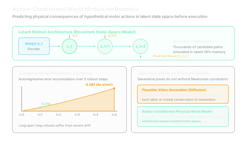
State-of-the-art robot world models (such as Recurrent State-Space Models or RSSMs) operate in a compressed latent space rather than predicting raw pixel grids at every step:

1[Observation o_t] ──> [Encoder] ──> [Latent State s_t]2                                          │3                                   [Action a_t]4                                          │5                                          ▼6                                   [Transition Model] ──> [Latent State s_{t+1}] ──> [Predictor: Reward / Values]7                                                                  │8                                                           [Action a_{t+1}]9                                                                  │10                                                                  ▼11                                                           [Latent State s_{t+2}]

1. Latent State-Space Transitions

Instead of running a heavy diffusion decoder to reconstruct a $256 \times 256$ RGB image at every simulated microsecond, the model maps observation $o_t$ into a compact latent vector $\mathbf{s}_t \in \mathbb{R}^d$ .

The transition model $p_\theta(\mathbf{s}_{t+1} \mid \mathbf{s}_t, \mathbf{a}_t)$ predicts the next latent state conditioned on current latent state $\mathbf{s}_t$ and executed motor action $\mathbf{a}_t$ . Because latent transitions involve simple matrix multiplications and small MLP/recurrent layers, a GPU can roll out thousands of parallel 15-step trajectories in a few milliseconds.

2. Autoregressive Error Compounding

When a robot uses its world model to plan multiple steps into the future without receiving fresh camera observations, predictions are made autoregressively: step $t+1$ depends on predicted step $t$ , step $t+2$ depends on predicted step $t+1$ , and so forth.

Every single step prediction introduces an error with variance $\sigma_\epsilon^2$ . In a dynamic system where future state sensitivity is governed by transition Jacobian $A$ , prediction variance compounds exponentially.

For a simplified 1D system $x_{t+1} = A x_t + B u_t + \epsilon_t$ , with independent noise $\operatorname{Var}(\epsilon_t) = \sigma_\epsilon^2$ , the cumulative variance $\Sigma_t = \operatorname{Var}(x_t \mid x_0)$ after $t$ ungrounded imagination steps is:

\Sigma_t = A^2 \Sigma_{t-1} + \sigma_\epsilon^2

Expanding this recurrence from initial known state $\Sigma_0 = 0$ :

\Sigma_t = \sigma_\epsilon^2 \sum_{k=0}^{t-1} A^{2k} = \sigma_\epsilon^2 \left( 1 + A^2 + A^4 + \dots + A^{2(t-1)} \right)

If $A > 1$ (an unstable or highly sensitive physical regime, such as balancing an inverted pendulum or handling slippery contact), prediction uncertainty explodes rapidly, causing long-horizon imagined plans to fail when executed on real hardware.

3. Worked Example: Compounding Uncertainty in a 5-Step Rollout

Consider an autonomous mobile manipulator using a world model to evaluate a candidate pushing trajectory over a 5-step horizon.

Transition sensitivity factor: $A = 1.05$ .
Single-step transition error variance: $\sigma_\epsilon^2 = 0.010\text{ m}^2$ (standard deviation $\sigma_\epsilon = 0.100\text{ m} = 10\text{ cm}$ ).
$A^2 = (1.05)^2 = 1.1025$ .

Compute cumulative variance $\Sigma_t$ at each step of the rollout:

Step 1: $\Sigma_1 = \sigma_\epsilon^2 = 0.0100\text{ m}^2 \quad (\sigma_1 = 0.1000\text{ m})$
Step 2: $\Sigma_2 = 1.1025 \times 0.0100 + 0.0100 = 0.011025 + 0.0100 = 0.0210\text{ m}^2 \quad (\sigma_2 \approx 0.1450\text{ m})$
Step 3: $\Sigma_3 = 1.1025 \times 0.021025 + 0.0100 = 0.02318 + 0.0100 = 0.0332\text{ m}^2 \quad (\sigma_3 \approx 0.1822\text{ m})$
Step 4: $\Sigma_4 = 1.1025 \times 0.03318 + 0.0100 = 0.03658 + 0.0100 = 0.0466\text{ m}^2 \quad (\sigma_4 \approx 0.2158\text{ m})$
Step 5: $\Sigma_5 = 1.1025 \times 0.04658 + 0.0100 = 0.05135 + 0.0100 = 0.0614\text{ m}^2 \approx 0.061\text{ m}^2 \quad (\sigma_5 \approx 0.2477\text{ m})$

By step 5, cumulative uncertainty variance has ballooned from $0.010$ to $0.061$ —a $6.1\times$ increase in uncertainty. The spatial confidence interval ( $\pm 2\sigma$ ) expands from $\pm 20\text{ cm}$ at step 1 to nearly $\pm 50\text{ cm}$ at step 5.

This numerical explosion proves why robot planners cannot rely on open-loop 50-step imagination rollouts. Production systems use short prediction horizons ( $H \approx 5\text{--}10$ ) and continuously re-anchor latent state $s_t$ to real camera observations.

Code

The following Python script computes autoregressive rollout trajectories and calculates the cumulative variance growth across multi-step imagination horizons:

1from dataclasses import dataclass2from typing import List, Tuple3import numpy as np4
5
6@dataclass7class WorldModelRollout:8    step: int9    mean_state: float10    variance: float11    std_dev: float12
13
14def simulate_autoregressive_rollout(15    initial_state: float = 0.0,16    sensitivity_a: float = 1.05,17    control_gain_b: float = 0.10,18    single_step_variance: float = 0.010,19    actions: List[float] = None,20) -> List[WorldModelRollout]:21    """Simulates an autoregressive latent rollout tracking state mean and compounding variance."""22    if actions is None:23        actions = [1.0] * 524
25    trajectory: List[WorldModelRollout] = []26    x = initial_state27    sigma_cum = 0.028    a_sq = sensitivity_a ** 229
30    for t, u in enumerate(actions, start=1):31        # Update mean state32        x = sensitivity_a * x + control_gain_b * u33        # Update cumulative variance34        sigma_cum = a_sq * sigma_cum + single_step_variance35        std = np.sqrt(sigma_cum)36
37        trajectory.append(38            WorldModelRollout(39                step=t,40                mean_state=round(x, 4),41                variance=round(sigma_cum, 4),42                std_dev=round(std, 4),43            )44        )45
46    return trajectory47
48
49# Execute 5-step rollout matching worked example numbers50rollout = simulate_autoregressive_rollout()51
52for step_info in rollout:53    print(54        f"Step {step_info.step}: Var = {step_info.variance:.4f} m^2, "55        f"StdDev = {step_info.std_dev:.4f} m"56    )57
58# Verify step 1 and step 5 match worked calculations59assert rollout[0].variance == 0.010060assert abs(rollout[4].variance - 0.0614) < 1e-361print(f"Variance grew {rollout[4].variance / rollout[0].variance:.2f}x over 5 steps.")

Watch Out For

Allowing the policy optimizer to exploit model hallucinations ('model exploitation')

Neural network world models are imperfect approximations of physics. During imagination planning, an optimizer searches for action sequences that maximize predicted reward.

The symptom is the policy discovering "physics loopholes": in the latent world model, vibrating a joint back and forth at $100\text{ Hz}$ might cause the predicted latent state to teleport forward without collision, yielding massive simulated rewards. When executed on the real robot, the arm simply shakes violently in place. Fix this by penalizing out-of-distribution actions, training ensembles of world models and using conservative lower-bound value estimates, or enforcing physical consistency losses during world model training.

Confusing pixel reconstruction loss with task-relevant dynamics fidelity

Practitioners often train world models by optimizing Mean Squared Error (MSE) or perceptual loss on reconstructed camera frames.

The symptom is the world model accurately reconstructing the static background wallpaper and sunlight shadows across the room, but completely ignoring the position of a tiny 2-centimeter bolt on the table because the bolt represents only 0.05% of total image pixels. Fix this by training world models with reward-prediction heads, contrastive latent dynamics objectives (such as DreamerV3 or PlaNet), or spatial-attention weighting that forces the latent state to prioritize contact and manipulation interfaces.

The Quick Version

Robot world models learn predictive simulators of physical dynamics from camera and proprioceptive interaction data.
Unlike passive video generators, physical world models condition predictions on commanded actions ( $\mathbf{a}_t$ ) and enforce physical causality.
Operating in a compact latent state-space ( $s_t$ ) allows GPUs to simulate thousands of parallel candidate rollouts in milliseconds for Model Predictive Control.
Autoregressive rollout error compounds: a 5-step rollout with sensitivity $A = 1.05$ and step variance $\sigma^2 = 0.010$ sees cumulative variance grow $6.1\times$ to $0.061\text{ m}^2$ .
Because ungrounded predictions drift rapidly, practical physical AI systems keep imagination horizons short ( $5\text{--}15$ steps) and continuously re-anchor to real sensor streams.