Robot Operational-Space Dynamics
A tool can feel heavier in one direction than another. Joint inertia and geometry together determine how a force at the tool becomes acceleration.
Why Does This Exist?
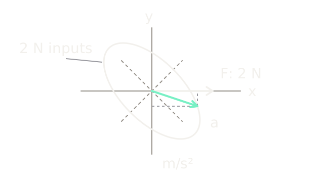
Push a robot tool right and it can initially accelerate right and down. That isn't a violation of Newton's law: the robot is a coupled mechanism with direction-dependent inertia. Operational-space dynamics expresses that inertia and the other dynamic loads in task coordinates, such as the tool's horizontal and vertical position.
The Jacobian maps joint velocity to tool velocity and tool force to joint effort. That kinematic mapping alone doesn't determine acceleration. Joint dynamics supplies the missing mass matrix. Combining them distinguishes an easy geometric direction from an easy acceleration direction.
Think of It Like This
Pushing a tray on two crossed sliding rails
One rail moves a heavy carriage; the other moves a lighter carriage. Rotate both rails relative to the room. A room-right push has components along both rails, but the lighter direction accelerates more. Adding those motions can tilt the resulting acceleration away from your push. Rails map to joint directions, carriage loads to joint inertia, and the room to task coordinates. The analogy stops at changing geometry: our rails stay fixed, while an arm's Jacobian and inertia change with posture.
How It Actually Works
Combine geometry and inertia at one state
Let collect joint coordinates, task position, and the translational Jacobian. Then and
Use , where is joint inertia, collects gravity, velocity and modelled friction loads, and is applied joint effort. At this stage there are no additional contact constraints. For a task-force contribution applied through , substitution gives
+\underbrace{\dot J\dot q-JM^{-1}h}_{a_0}.$$ $W$ is task mobility, $a_0$ the acceleration without that force contribution, and $T$ denotes transpose. When $J$ has independent rows and $M$ is positive definite, task inertia is $\Lambda=W^{-1}$. Thus $F=\Lambda(\ddot x-a_0)$. Compute linear solves rather than explicitly forming inverses in software. [Modern Robotics' task-space derivation](https://modernrobotics.northwestern.edu/nu-gm-book-resource/8-6-dynamics-in-the-task-space/) explains the equivalent dynamic equation for an invertible Jacobian, including velocity and gravity terms. In that square case, $\Lambda=J^{-T}MJ^{-1}$. The mobility expression above also handles redundant, fully actuated systems for the selected independent task coordinates. ### Work a rotated two-axis slide Take two orthogonal prismatic joints, so both joint coordinates $q_1,q_2$ are translations in metres. They form a horizontal planar slide, rotated 45° counterclockwise relative to fixed room axes $x$ right and $y$ up **in the drawing**. This is a top view; $y$ is not gravitational height. Stipulate effective joint inertia $M=\operatorname{diag}(2,1)$ kg, constant geometry, zero initial velocity, and no friction or in-plane gravity. These are synthetic effective moving masses, not motor rotor inertias. The constant Jacobian is the rotation $$J=\frac1{\sqrt2}\begin{bmatrix}1&-1\\1&1\end{bmatrix}.$$ The first joint direction is room northeast; the second is northwest. Since $J$ is orthogonal, $J^{-1}=J^T$. Multiplication gives $$\Lambda=JMJ^T=\begin{bmatrix}1.5&0.5\\0.5&1.5\end{bmatrix}\ \mathrm{kg},\quad W=\begin{bmatrix}0.75&-0.25\\-0.25&0.75\end{bmatrix}\ \mathrm{kg}^{-1}.$$ Apply $F=(2,0)^T$ N. Joint efforts are $J^TF=(\sqrt2,-\sqrt2)^T$ N. Dividing by the joint masses gives $\ddot q=(1/\sqrt2,-\sqrt2)^T$ m/s². Rotate back: $$\ddot x=WF=(1.5,-0.5)^T\ \mathrm{m/s^2}.$$ The angle below room-right is $\arctan(0.5/1.5)=18.435^\circ$. Conversely, to obtain desired acceleration $(1,0)^T$ m/s², the necessary task force is $\Lambda(1,0)^T=(1.5,0.5)^T$ N. A pure horizontal acceleration requires an upward **in-plane** force component to offset the coupled response. The SVG plots acceleration vectors from a common origin, not a physical displacement path. The ellipse contains accelerations from all task forces of magnitude 2 N. Its principal semiaxes are 1 and 2 m/s², along the heavy and light joint directions respectively. It uses 60 drawing units per m/s². The white force arrow uses a separate scale of 60 drawing units per newton; compare directions, not lengths across units. The mint acceleration arrow ends at $(1.5,-0.5)$, exactly on the ellipse. Dashed projections expose its nonzero vertical component. ### What changes for an arm or a redundant task? [The mass-matrix explanation](https://modernrobotics.northwestern.edu/nu-gm-book-resource/8-1-3-understanding-the-mass-matrix/) shows force and acceleration ellipsoids and their principal directions. In a moving arm, retaining $\dot J\dot q$ is essential: constant joint speed can produce curved tool motion and nonzero acceleration. Subtracting gravity without the velocity terms is only a restricted compensation scheme. If the selected task loses rank, $W$ is singular and an ordinary inverse $\Lambda$ does not exist. Damping limits numerical amplification but changes the requested dynamics. For a redundant full-row-rank task, the inertia-weighted inverse $\bar J=M^{-1}J^T\Lambda$ satisfies $J\bar J=I$, where $I$ is the task identity matrix. It supplies joint accelerations $\bar J(\ddot x_d-\dot J\dot q)$ for a desired task acceleration $\ddot x_d$. Additional null-space motion still needs consistent dynamics and limits. A kinematic null-space velocity projector is not automatically a torque-decoupling projector; [redundancy and null-space control](/concepts/physical-ai/robot-redundancy-and-null-space-control) explains that distinction. Contact and floating-base underactuation require constrained dynamics rather than blindly reusing the fixed-base equation. Likewise, a full six-dimensional wrench mixes force and moment, so translational ellipse lengths cannot be compared directly with angular ones without a declared scaling. Use task-space dynamics when shaping tool acceleration or force response matters. It buys interpretable task behavior at the cost of inertia estimation, fast solves and handling weak directions. For a slow pose reach where effort is irrelevant, kinematics can answer the simpler question with fewer modelling assumptions. ## Code This NumPy example follows force through joint effort and joint acceleration, checks the independent task solve, and verifies equal kinetic energy in both coordinate descriptions. ```python import numpy as np def task_mobility(J: np.ndarray, M: np.ndarray) -> np.ndarray: return J @ np.linalg.solve(M, J.T) J = np.array([[1.0, -1.0], [1.0, 1.0]]) / np.sqrt(2) M = np.diag([2.0, 1.0]) W = task_mobility(J, M) inertia = np.linalg.solve(W, np.eye(2)) force = np.array([2.0, 0.0]) joint_force = J.T @ force joint_accel = np.linalg.solve(M, joint_force) accel = J @ joint_accel assert np.allclose(accel, W @ force) assert np.allclose(accel, [1.5, -0.5]) velocity = np.array([0.3, -0.2]) joint_velocity = np.linalg.solve(J, velocity) assert np.isclose(velocity @ inertia @ velocity, joint_velocity @ M @ joint_velocity) print("task acceleration:", np.round(accel, 4)) print("force for horizontal unit acceleration:", np.round(inertia @ np.array([1.0, 0.0]), 4)) ``` Output vectors are `[ 1.5 -0.5]` m/s² and `[1.5 0.5]` N. Kinetic energy is half the checked quadratic form. No changing Jacobian, actuator saturation or contact is simulated. ## Watch Out For <PitfallCard title="Tool force is mapped to torque without an inertia model"> $J^TF$ correctly maps effort, but doesn't imply that acceleration points along $F$. Include $M$ and acceleration bias when predicting the response. The worked horizontal force produces a downward acceleration component even with perfect calibration and unlimited actuators. </PitfallCard> <PitfallCard title="A singular task is treated as a very heavy tool"> Near rank loss, numerical task inertia can become enormous or unreliable. Inspect the selected task directions and scaled singular values. Reduce the task, change posture or use an explicitly damped design; a raw inverse cannot create missing motion authority. </PitfallCard> ## The Quick Version - Task inertia combines joint inertia and the Jacobian through $\Lambda=(JM^{-1}J^T)^{-1}$ when the selected task has full row rank. - Force and acceleration generally align only along principal inertia directions. - The worked 2 N horizontal force gives acceleration $(1.5,-0.5)$ m/s². - Moving robots require velocity and gravity terms as well as the instantaneous mass matrix. - Singular tasks, contact constraints and underactuated bases require additional treatment.