Robot Redundancy and Null-Space Control

An arm can move its elbow while keeping its hand still. Null-space control coordinates spare joint motion so it does not change the primary tool velocity at the current pose.

Three nonzero joint rates produce endpoint-velocity contributions that close into a zero-sum triangle.

Why Does This Exist?

Keeping a tool on target doesn't determine every joint angle of a redundant arm. A controller still needs to choose a posture: perhaps to move away from a joint limit or keep an elbow clear of nearby equipment. Null-space control gives that secondary motion a place to act without changing the primary task's instantaneous velocity.

A Jacobian maps small joint rates to tool velocity. A null-space vector is a set of rates that the map sends to zero. Redundancy is relative to the chosen task: three planar joints are redundant for two-dimensional tool position, but generally not for position plus orientation. The mathematical foundation is vector spaces and rank.

Think of It Like This

Keeping a tray's mark over a floor tile

Hold a tray so a marked point stays above one floor tile. You can coordinate your shoulder, elbow and wrist to change your posture while keeping that point in place. The point is the primary task; comfortable joint positions are the secondary goal; coordinated posture changes are self-motion.

Keeping one point fixed doesn't also keep the tray level. That is the analogy's useful limit: adding orientation to the task consumes freedom that position alone leaves available.

How It Actually Works

Separate the requested tool motion from posture motion

Let $q$ be the joint-position vector and $J(q)$ the task Jacobian. Then $\dot x=J\dot q$ , with $\dot x$ the selected tool velocity and $\dot q$ the joint rates. At full row rank, the minimum Euclidean-norm solution uses the pseudoinverse

J^+=J^T(JJ^T)^{-1}.

For desired task velocity $v$ , all solutions can be written

\dot q=J^+v+Nz,\qquad N=I-J^+J.

$I$ is the joint-space identity matrix, $z$ is a proposed secondary joint-rate vector, and $N$ projects it into the Jacobian's null space. Because $JN=0$ and $JJ^+=I$ under this rank assumption, multiplying by $J$ recovers $v$ . Modern Robotics' redundant-arm example distinguishes this family of joint solutions from rank loss at a singularity.

For example, with a posture cost $H(q)$ , choose $z=-k\nabla H$ where $k$ is a positive gain with suitable units. The projection retains only the part of that proposed motion compatible with the primary task. It can remove the entire proposal. Honegger and Codourey's redundancy-resolution paper, Section 3.2, gives the pseudoinverse-plus-null-space construction and weighted alternatives.

Worked example: a real three-link geometry

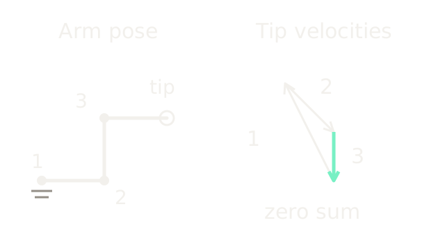
Take a planar arm with three one-metre links and relative joint angles $q=(0,\pi/2,-\pi/2)$ radians. Its successive joints are at $(0,0)$ , $(1,0)$ and $(1,1)$ m; the tip is $(2,1)$ m. For rotation about a planar joint at $(x_i,y_i)$ , the tip-velocity column is $(-(y-y_i),x-x_i)^T$ . Therefore

J=\begin{bmatrix}-1&-1&0\\2&1&1\end{bmatrix},\qquad n=(1,-1,-1)^T,\qquad Jn=0.

Here $n$ spans the one-dimensional null space, so $N=nn^T/(n^Tn)=nn^T/3$ . Suppose a posture objective proposes $z=(0.3,0,0)$ rad/s. Its projection is $Nz=(0.1,-0.1,-0.1)$ rad/s. The three tip-velocity contributions are

(-0.1,0.2)+(0.1,-0.1)+(0,-0.1)=(0,0)\ \mathrm{m/s}.

The drawing shows the exact arm pose on the left. On the right, head-to-tail vectors form a closed triangle; the highlighted final edge closes the sum. It is a vector-addition inset, not a second arm configuration or a traced tip path.

If the primary tool request becomes $v=(0.1,0)$ m/s, its minimum-norm joint rates are $(0,-0.1,0.1)$ rad/s. Adding our projected posture motion gives $(0.1,-0.2,0)$ rad/s. Direct substitution yields $J\dot q=(0.1,0)$ m/s. The same extra motion now coexists with a moving tool.

Why doesn't one projection solve the whole trajectory?

The matrix depends on the current configuration. Integrating the stationary-tool rates as one fixed Euler step for $0.1$ s moves the true nonlinear endpoint by approximately $0.000100$ m. A $0.01$ s step gives about $0.000001$ m. The command cancels the first-order velocity, leaving second-order position error. Recompute the Jacobian as the robot moves and close the loop on measured task error; this example freezes the rates precisely to expose the limitation.

Near a singularity, an exact pseudoinverse may demand large joint rates. Damping reduces that demand but replacing $J^+$ by a damped inverse generally makes $J(I-J^\#J)$ nonzero: secondary motion can leak into the primary task. Likewise, clipping individual rates after solving can break cancellation. When hard limits matter, solve a constrained velocity problem and explicitly decide which task can relax. A soft posture cost is not a joint-limit guarantee.

Redundancy buys posture choice at the cost of extra optimization and task-priority decisions. A velocity projector also does not establish torque-level decoupling. Dietrich's treatment of projection consistency, Chapter 4, distinguishes kinematic and dynamic hierarchy requirements. If the task already consumes every independent joint direction, there may be no secondary freedom to use.

Operational-space dynamics combines the Jacobian with joint inertia and introduces the inertia-weighted inverse. That is the next step when a secondary effort must preserve task acceleration rather than only task velocity.

Code

This standard-library check projects the posture proposal, verifies both velocity tasks, and evaluates the actual nonlinear forward kinematics after finite steps.

1from math import cos, dist, isclose, pi, sin2
3Vec = tuple[float, float, float]4J = ((-1.0, -1.0, 0.0), (2.0, 1.0, 1.0))5n: Vec = (1.0, -1.0, -1.0)6
7def project(z: Vec) -> Vec:8    scale = sum(a*b for a, b in zip(n, z)) / sum(a*a for a in n)9    return tuple(scale*a for a in n)10
11def tool_velocity(rates: Vec) -> tuple[float, float]:12    return tuple(sum(a*b for a, b in zip(row, rates)) for row in J)13
14def tip(q: Vec) -> tuple[float, float]:15    angle = x = y = 0.016    for joint in q:17        angle += joint18        x, y = x + cos(angle), y + sin(angle)19    return x, y20
21q: Vec = (0.0, pi/2, -pi/2)22posture = project((0.3, 0.0, 0.0))23assert all(isclose(x, 0.0, abs_tol=1e-14) for x in tool_velocity(posture))24combined = tuple(a+b for a, b in zip((0.0, -0.1, 0.1), posture))25assert all(isclose(a, b, abs_tol=1e-14)26           for a, b in zip(tool_velocity(combined), (0.1, 0.0)))27for dt in (0.1, 0.01):28    stepped = tuple(a+dt*b for a, b in zip(q, posture))29    print(f"dt={dt:.2f}: endpoint drift={dist(tip(q), tip(stepped)):.9f} m")

Output: dt=0.10: endpoint drift=0.000099999 m and dt=0.01: endpoint drift=0.000001000 m.

Watch Out For

Position redundancy is mistaken for full-pose redundancy

The endpoint stays put but the tool twists. The Jacobian constrained only position. Include the required orientation components before computing rank and null space; the three-link fixture then generally loses its one free direction.

A final rate clamp destroys the primary task

The unconstrained command has zero tip velocity, but one saturated joint leaves an uncancelled contribution. Put actuator limits into the solve rather than assuming postprocessing preserves the projection. Monitor the executed task residual after any filtering or rate limiting.

The Quick Version

Redundancy depends on the selected task and the Jacobian's rank, not joint count alone.
The exact projector $I-J^+J$ keeps secondary joint motion out of the current task velocity.
The worked arm's three nonzero velocity contributions cancel, while finite frozen-rate steps still cause nonlinear position drift.
Damping, clipping and torque dynamics change the guarantees of a purely kinematic projection.