Robot Trajectory Generation and Time Scaling

A path says where a robot should go; a trajectory says when it should be there. The clock must leave enough room for speed, acceleration and jerk limits.

Stretching the same quintic move lowers its peak speed below the limit.

Why Does This Exist?

A collision-free arm path can still demand an impossible jump in speed at its next waypoint. Trajectory generation turns geometric intent into position, velocity and acceleration references indexed by time. A controller then attempts to track those references within the hardware's actual capabilities.

Motion planning finds a route through admissible configurations. A path $q(s)$ describes that route using progress $s$ from zero to one. A time scaling $s(t)$ decides how progress changes with time. Their composition $q(s(t))$ is a trajectory. Modern Robotics on paths and trajectories establishes this separation. This page works a smooth joint move and tests its derivative limits; it doesn't search around obstacles.

Think of It Like This

A train route and its driving schedule

The rails determine where a train can go. Its driving schedule determines when it reaches each point, how quickly it gains speed and when it brakes. Sending the same train along the same rails faster demands more acceleration. A sharp bend cannot be made physically gentle merely by writing a smooth-looking timetable.

The rails map to the path and the schedule to time scaling. The analogy stops at robot geometry: joint-space lines needn't produce straight tool motion, and moving obstacles can make the same route clear at one time but blocked at another.

How It Actually Works

Which derivatives must stay bounded?

Let $q$ be joint angle in radians and $t$ time in seconds. Velocity $\dot q$ is the rate of position change, acceleration $\ddot q$ the rate of velocity change, and jerk $\dddot q$ the rate of acceleration change. They have units rad/s, rad/s² and rad/s³. A continuous position can still hide a velocity jump.

For a differentiable path, the chain rule gives

\dot q=q'(s)\dot s,\qquad \ddot q=q'(s)\ddot s+q''(s)\dot s^2.

Primes mean derivatives with respect to path progress, while dots mean time derivatives. Curvature contributes through $q''(s)\dot s^2$ . At a geometric corner the tangent changes abruptly, so a bounded-acceleration trajectory must stop there or replace the corner with a checked smooth path. Retiming cannot erase the corner.

Build a rest-to-rest quintic

For one straight joint-space segment, let $q_0$ and $q_f$ be start and finish angles, $\Delta q=q_f-q_0$ their difference, $T>0$ the finishing time and $r=t/T$ normalized time. Use

q(t)=q_0+\Delta q\,s(r),\qquad s(r)=10r^3-15r^4+6r^5.

This quintic, a polynomial of degree five, satisfies $s(0)=0$ , $s(1)=1$ and zero first and second derivatives at both ends. Differentiation gives

s'(r)=30r^2(1-r)^2,\quad s''(r)=60r-180r^2+120r^3,\quad s'''(r)=60-360r+360r^2.

Thus $\dot q=\Delta q\,s'/T$ , $\ddot q=\Delta q\,s''/T^2$ , and $\dddot q=\Delta q\,s'''/T^3$ . Stretching the clock by factor $c$ divides velocity by $c$ , acceleration by $c^2$ and jerk by $c^3$ , while retaining the path. Modern Robotics on time scalings compares quintic, cubic, trapezoidal and S-curve constructions.

Check a move against three limits

Take the synthetic move $q_0=0$ , $q_f=1$ radian. Set allowed magnitudes to $v_{max}=0.8$ rad/s, $a_{max}=1.5$ rad/s² and $j_{max}=10$ rad/s³. The derivatives above give exact peak magnitudes

v_{peak}=\frac{15|\Delta q|}{8T},\qquad a_{peak}=\frac{10|\Delta q|}{\sqrt3\,T^2},\qquad j_{peak}=\frac{60|\Delta q|}{T^3}.

The speed peaks at $r=1/2$ . Acceleration extrema occur at $r=(3\pm\sqrt3)/6$ , where jerk is zero. Maximum absolute jerk occurs at an endpoint. Solving each inequality for $T$ gives

T\geq\max\left( \frac{15|\Delta q|}{8v_{max}}, \sqrt{\frac{10|\Delta q|}{\sqrt3\,a_{max}}}, \sqrt[3]{\frac{60|\Delta q|}{j_{max}}}\right).

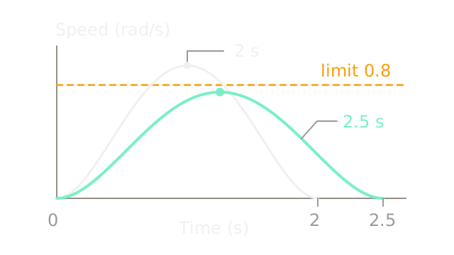
Our three bounds are approximately $2.34375$ , $1.961887$ and $1.817121$ seconds. Speed is the binding constraint. With $T=2$ s, peak speed is $0.9375$ rad/s, which violates the limit, despite peak acceleration $1.443376$ rad/s² and jerk $7.5$ rad/s³ passing their limits. Choose $T=2.5$ s: peaks become $0.75$ rad/s, $0.923760$ rad/s² and $3.84$ rad/s³. All three pass this reference-motion check.

The diagram plots both speed profiles on shared axes. Each curve encloses the same one-radian displacement; the longer move spreads it over more time. The dashed amber line is the speed bound, not an acceleration limit. The two maxima occur at different times because both occur halfway through their own moves.

What changes on a complete robot?

For a multi-joint straight segment, compute these bounds for every moving joint and choose a common $T$ that satisfies all of them. A shared $s(t)$ preserves the planned joint-space line. Choosing a separate clock for each joint changes the path and may lose collision clearance. A joint-space line also doesn't guarantee straight tool travel.

The quintic starts and ends with zero acceleration, but its endpoint jerk is nonzero. Joining it to a stationary hold creates a jerk jump, not an infinite jerk impulse: acceleration remains continuous. A requirement for continuous jerk or for nonzero boundary velocities needs a different construction. A time-optimal, jerk-bounded generator solves another problem; this fixed quintic only provides a convenient feasible reference when its checks pass.

Interpolation is part of execution. The ROS trajectory representation documentation distinguishes position-only linear interpolation from cubic and quintic interpolation with derivative data. Supplying only positions can change the reference's continuity. Check the actual controller interface and interpolated trajectory, rather than only the offline samples.

Dynamics adds torque requirements, gravity and coupled loads. A reference passing derivative limits can still exceed a torque limit. Moving obstacles, tracking error and contact require additional checks. Use simple retiming for a fixed admissible path; use replanning when the route itself must change.

Code

This code computes analytic bounds rather than sampling a curve and hoping the samples catch its extrema. It also rejects the tempting two-second setting.

1from math import sqrt2
3def peaks(delta: float, total: float) -> tuple[float, float, float]:4    if total <= 0:5        raise ValueError("positive finishing time required")6    distance = abs(delta)7    return (1.875 * distance / total,8            10 * distance / (sqrt(3) * total**2),9            60 * distance / total**3)10
11def required_time(delta: float, v: float, a: float, j: float) -> float:12    if min(v, a, j) <= 0:13        raise ValueError("positive limits required")14    distance = abs(delta)15    return max(1.875 * distance / v,16               sqrt(10 * distance / (sqrt(3) * a)),17               (60 * distance / j)**(1 / 3))18
19limits = (0.8, 1.5, 10.0)20minimum = required_time(1.0, *limits)21assert peaks(1.0, 2.0)[0] > limits[0]22assert all(p <= bound for p, bound in zip(peaks(1.0, 2.5), limits))23assert peaks(-1.0, 2.5) == peaks(1.0, 2.5)24print(f"minimum for this quintic: {minimum:.5f} s")25print(tuple(round(x, 6) for x in peaks(1.0, 2.5)))

Output: minimum for this quintic: 2.34375 s and (0.75, 0.92376, 3.84). This minimum is specific to the chosen quintic family and derivative bounds, not a global minimum over all possible trajectories.

Watch Out For

Every waypoint passes, but the interpolated move fails

A plotted sample sequence stays within limits while its interpolating polynomial overshoots between samples. Check continuous-segment extrema and the interpolation actually executed by the controller. Clipping a reference afterward changes its derivatives and can destroy synchronization between joints.

A new target restarts a rest-to-rest polynomial mid-motion

The measured joint is moving when a new segment assumes zero starting velocity. Its reference velocity jumps at the handoff. Initialize a boundary-value trajectory from the intended current position, velocity and acceleration, or use a generator that handles online target changes with explicit limits and a defined stop behavior.

The Quick Version

A path fixes geometry; a time scaling turns it into a time-indexed trajectory.
Quintic rest-to-rest interpolation gives zero endpoint velocity and acceleration.
Smoothness doesn't prove feasibility: compute speed, acceleration and jerk extrema.
A shared clock preserves a multi-joint path; independent retiming can change it.
Derivative limits, torque limits and collision clearance are separate requirements.