Go-Explore
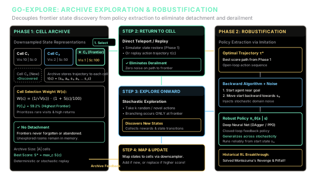
Go-Explore breaks hard exploration into two phases: first discovering new states by systematically archiving and returning to promising frontiers, then training a robust policy to reproduce the best trajectory.
Why Does This Exist?
In reinforcement learning, environments with sparse, delayed rewards and long-horizon bottlenecks represent the hardest exploration benchmark. For years, benchmark Atari games like Montezuma's Revenge and Pitfall! defeated state-of-the-art model-free RL algorithms, including Deep Q-Networks (DQN), Proximal Policy Optimization (PPO), Rainbow, and distributed actor-critic architectures. Even intrinsic motivation mechanisms—such as prediction-error curiosity (ICM) or count-based exploration bonuses—struggled to achieve consistent progress across multi-room mazes.
Standard reinforcement learning methods fail in these environments because they fundamentally couple state space exploration with policy optimization. When an agent relies on standard exploratory noise (such as -greedy action selection, Gaussian perturbations, or policy entropy bonuses) while simultaneously updating its policy parameters, it falls prey to two fatal exploration pathologies:
- Detachment: An agent's exploratory policy discovers a promising frontier (e.g., reaching the entrance of a second room). However, as the agent explores the local neighborhood, its intrinsic novelty bonuses rapidly diminish. Before the agent can fully exhaust the frontier, policy parameter updates or environment non-stationarity cause it to wander away. Because standard RL stores knowledge solely in neural network weights rather than an explicit state archive, the agent forgets how to reach that frontier and rarely rediscovers it.
- Derailment: To reach a deeply nested frontier state at depth in a complex environment, the agent must execute a precise, coordinated sequence of 100 actions (e.g., jumping across conveyor belts, dodging rolling skulls, and timing rope swings). If the exploration mechanism injects exploratory stochasticity at every step along the way, the probability of executing the precise trajectory collapses exponentially. The exploratory noise meant to discover new states inevitably derails the agent before it can even return to the frontier!
Introduced by Ecoffet et al. (Nature 2021), Go-Explore solves this fundamental dilemma by separating exploration into two distinct phases:
- Phase 1 (Explore Until Solved): Build an explicit archive of discovered environmental states. Instead of exploring from the initial start state every episode, the agent selects a promising cell from the archive, returns directly to that exact state without exploratory noise, and only then explores onward.
- Phase 2 (Robustification): Once a high-scoring trajectory is discovered, extract a robust, closed-loop deep neural network policy via imitation learning and domain randomization so the agent can execute the solution from scratch under stochastic environmental noise.
Think of It Like This
The Labyrinth Surveyor's Teleportation Map
Imagine an ancient, subterranean labyrinth filled with hundreds of dark corridors, locked iron gates, and treacherous pitfalls:
-
The Standard RL Adventurer: Every morning, the adventurer respawns at the labyrinth entrance gate (). They start sprinting through corridors they already mapped. However, because they are instructed to "stay curious," they randomly stumble, make wrong turns, and trip into traps along corridors they mastered days ago (derailment). If they ever happen to stumble upon a hidden staircase to the third level, they wander around for ten minutes, find no immediate gold, and leave. By next week, the adventurer has completely forgotten which hallway led to that staircase (detachment).
-
The Go-Explore Surveyor: The Go-Explore surveyor carries a detailed parchment archive and a teleportation beacon:
- Step 1 (Select): Every morning, the surveyor opens the archive and picks the most promising, underexplored frontier room mapped so far—prioritizing rooms that were rarely visited but produced high rewards.
- Step 2 (Return): Instead of running through all the solved hallways, the surveyor uses the beacon to teleport directly into that frontier room. Not a single step is wasted, and no random stumbling occurs during transit.
- Step 3 (Explore): Once safely inside the frontier room, the surveyor steps into the darkness, taking 10 bold, exploratory steps into uncharted territory.
- Step 4 (Archive): If any newly discovered rooms are found, the surveyor logs their floor plan and the exact steps taken to reach them into the archive.
- Phase 2 (The Marathon Runner): Once the surveyor discovers the labyrinth's master treasure room, they train an elite runner to sprint the entire path from the entrance gate to the treasure vault, drilling them under falling rocks and slippery floors until the path is executed flawlessly from start to finish.
Where the analogy stops: In physical labyrinths, rooms have clean structural walls. In video games and robotic tasks, raw environmental states consist of continuous visual frames ( pixels). Teleporting requires either restoring simulator memory checkpoints or deterministically replaying action sequences, while grouping visual frames into distinct "rooms" requires downsampling and representation mapping.
How It Actually Works
Detachment, Derailment, and the Two-Phase Exploration Paradigm
Go-Explore formalizes environment navigation as a search process over an expanding discrete cell archive , decoupling search tree expansion from policy representation.
+-------------------------------------------------------------------------------+| PHASE 1: EXPLORE UNTIL SOLVED || || +-------------------+ 1. Select +-------------------+ || | Cell Archive | -----------> | Return to Cell | (No noise added; || | A_archive = {c} | | without drift | derailment cured) || +-------------------+ +-------------------+ || ^ | || | 4. Map & | 2. Reached frontier || | Update v || | +-------------------+ || +----------------------- | Explore Onward | (k steps of || (Detachment cured) | from frontier | stochastic noise) || +-------------------+ |+-------------------------------------------------------------------------------+ | | Discovered Winning Trajectory tau* v+-------------------------------------------------------------------------------+| PHASE 2: ROBUSTIFICATION || || Trajectory tau* ----> Backward Algorithm ----> Deep Policy pi_theta(a | s) || (Open-loop path) + Environmental Noise (Closed-loop neural net) |+-------------------------------------------------------------------------------+1. Cell Representation and Archive Structure
Let denote a high-dimensional observation (e.g., an Atari frame). A downsampling function maps to a discrete cell identifier (for example, downsampling an image to grayscale pixels with 8 intensity levels).
The archive maps each discovered cell to a tuple: where:
- is the stored action trajectory leading from start state to cell .
- is the cumulative visitation count (the number of times cell has been chosen for exploration).
- is the cumulative environment return achieved upon reaching cell .
- is the underlying environment simulator state for cell .
2. Phase 1: The Four-Step Discovery Loop
The agent repeats four core steps until the environment is solved or a computation budget is exhausted:
-
Step A — Select a Promising Cell: A cell is sampled from the archive according to a probability distribution proportional to an exploration weight : The heuristic weight function balances novelty (inversely proportional to visitation count) and task performance (proportional to cumulative score): where is a normalization constant. Cells that have been chosen fewer times receive higher weight, while cells that accumulated higher scores are prioritized to deepen promising branches.
-
Step B — Return to Cell: The agent travels to cell without exploratory noise:
- With simulator state reset: The simulator's internal state is restored directly to .
- Without simulator reset (action replay): In non-resettable environments, the agent resets to and deterministically replays the stored action sequence . Because zero exploratory stochasticity is injected during transit, the agent reaches the exact frontier state with reliability, completely eliminating derailment.
-
Step C — Explore Onward: From state , the agent executes exploratory actions (e.g., steps sampled from a uniform random action distribution or an intrinsic curiosity policy).
-
Step D — Map and Update Archive: At each step during exploration, the agent visits a state with cumulative score and trajectory . The state is mapped to cell .
- Novel Cell: If , add to the archive with , , and .
- Better Trajectory: If , compare with existing entry . If , or if and (a shorter path to the same state), replace the stored trajectory and score. Because all discovered cells remain permanently in , frontiers are never abandoned or forgotten, completely eliminating detachment.
3. Phase 2: Policy Robustification
Phase 1 produces an open-loop trajectory that achieves a high score, but open-loop sequences are brittle: if the test environment introduces stochastic transitions (e.g., sticky actions where actions are repeated with probability ), an open-loop sequence fails.
Phase 2 trains a closed-loop neural network policy to reproduce robustly:
- The Backward Algorithm: Training directly from across a 5,000-step trajectory suffers from severe credit assignment degradation. Instead, the agent is initialized near the end of (at step ), learning via reinforcement learning (e.g., PPO) or imitation learning (Behavioral Cloning / DAgger) to reach the goal from the final states.
- Progressive Unrolling: As the policy achieves high success from , the start position is moved backward along toward until the policy can reliably complete the full task from the initial state under stochastic noise.
Worked numerical example
Consider a 2D navigation gridworld with an archive containing three discovered cells:
The cells possess the following properties:
- Cell (Initial corridor): Visited times, cumulative score , trajectory length .
- Cell (Key chamber): Visited times, cumulative score , trajectory length .
- Cell (Deep frontier room): Visited time, cumulative score , trajectory length .
Let the score normalization scale be .
Step 1: Compute Cell Exploration Weights
We evaluate the exploration weight function:
-
For Cell :
-
For Cell :
-
For Cell :
Step 2: Compute Selection Probabilities
Summing the individual weights yields total archive weight:
The normalized selection probabilities are:
Cell dominates the selection probability () because its rare visitation count () and high score () designate it as the primary unexhausted frontier.
Step 3: Return, Explore, and Archive Update
- Return: The agent selects cell and deterministically replays its 15-step trajectory without exploratory noise, landing exactly at state .
- Explore: From state , the agent executes exploratory actions, reaching a newly discovered state and obtaining an additional reward of .
- Archive Update:
- The new state maps to novel cell .
- New trajectory length: steps.
- New cumulative score: .
- Cell is added to the archive with , , and .
- The visitation counter of selected cell increments from to .
Code
Below is a complete, self-contained Python implementation of the Go-Explore Phase 1 archive, selection weighting, deterministic return, exploratory stepping, and archive updates.
import mathfrom dataclasses import dataclassfrom typing import Dict, List, Optional, Tuple
@dataclassclass CellEntry: """Represents a discovered state in the Go-Explore archive.""" cell_id: str visitation_count: int score: float trajectory: List[int] state: Tuple[int, int]
class GoExploreArchive: """Manages Phase 1 cell archiving, selection weighting, and state exploration
for hard-exploration reinforcement learning environments. """
def __init__(self, score_scale: float = 100.0) -> None: self.archive: Dict[str, CellEntry] = {} self.score_scale = score_scale
def add_or_update( self, cell_id: str, score: float, trajectory: List[int], state: Tuple[int, int], initial_visits: int = 1, ) -> bool: """Adds a new cell or updates an existing entry if the new trajectory yields
a strictly higher score or an equal score with fewer steps. """ if cell_id not in self.archive: self.archive[cell_id] = CellEntry( cell_id=cell_id, visitation_count=initial_visits, score=score, trajectory=list(trajectory), state=state, ) return True
entry = self.archive[cell_id] if score > entry.score or ( math.isclose(score, entry.score) and len(trajectory) < len(entry.trajectory) ): entry.score = score entry.trajectory = list(trajectory) entry.state = state return True return False
def compute_cell_weights(self) -> Dict[str, float]: """Calculates selection weight W(c) = (1 / sqrt(visitation)) * (1 + score / S0).""" weights: Dict[str, float] = {} for cid, entry in self.archive.items(): inv_freq = 1.0 / math.sqrt(entry.visitation_count) score_factor = 1.0 + (entry.score / self.score_scale) weights[cid] = inv_freq * score_factor return weights
def compute_selection_probabilities(self) -> Dict[str, float]: """Calculates normalized selection probabilities across all archived cells.""" weights = self.compute_cell_weights() total_w = sum(weights.values()) return {cid: w / total_w for cid, w in weights.items()}
def select_cell(self, target_cell: Optional[str] = None) -> str: """Selects a cell from the archive, incrementing its visitation count.""" probs = self.compute_selection_probabilities() chosen = target_cell if target_cell is not None else max(probs, key=lambda k: probs[k]) self.archive[chosen].visitation_count += 1 return chosen
def return_to_cell(self, cell_id: str) -> Tuple[Tuple[int, int], List[int]]: """Phase 1 Step B: Deterministic return to frontier cell without exploratory noise.""" entry = self.archive[cell_id] return entry.state, list(entry.trajectory)
def run_go_explore_simulation() -> None: # Initialize archive with worked example data archive = GoExploreArchive(score_scale=100.0) archive.add_or_update("C1", score=0.0, trajectory=[0] * 5, state=(0, 1), initial_visits=10) archive.add_or_update("C2", score=50.0, trajectory=[0] * 10, state=(2, 3), initial_visits=2) archive.add_or_update("C3", score=100.0, trajectory=[0] * 15, state=(5, 5), initial_visits=1)
# Step 1: Compute weights and probabilities weights = archive.compute_cell_weights() probs = archive.compute_selection_probabilities() total_w = sum(weights.values())
print("--- Phase 1: Archive Cell Weights ---") for cid in ["C1", "C2", "C3"]: print(f"{cid}: Weight = {weights[cid]:.4f}, Prob = {probs[cid]:.4f}") print(f"Total Archive Weight: {total_w:.4f}")
# Step 2: Select frontier cell C3 and return chosen = archive.select_cell("C3") state, traj = archive.return_to_cell(chosen) print(f"\nSelected Cell: {chosen}") print(f"Returned to State: {state}, Trajectory Length: {len(traj)}")
# Step 3: Explore forward k=3 steps new_state = (state[0] + 1, state[1] + 2) new_score = archive.archive[chosen].score + 20.0 new_traj = traj + [1, 2, 0]
# Step 4: Archive update with novel cell C4 archive.add_or_update("C4", score=new_score, trajectory=new_traj, state=new_state, initial_visits=1)
c4_entry = archive.archive["C4"] c3_entry = archive.archive["C3"] print("\n--- Archive Update ---") print( f"Added Cell C4: Score = {new_score:.1f}, " f"Trajectory Length = {len(new_traj)}, Visited = {c4_entry.visitation_count}" ) print(f"C3 New Visitation Count: {c3_entry.visitation_count}")
# Step 5: Automated validation assertions assert math.isclose(weights["C1"], 0.3162, abs_tol=1e-3), "C1 weight mismatch" assert math.isclose(weights["C2"], 1.0607, abs_tol=1e-3), "C2 weight mismatch" assert math.isclose(weights["C3"], 2.0000, abs_tol=1e-3), "C3 weight mismatch" assert math.isclose(total_w, 3.3769, abs_tol=1e-3), "Total weight mismatch" assert math.isclose(probs["C3"], 0.5923, abs_tol=1e-3), "C3 selection probability mismatch" assert len(archive.archive) == 4, "Archive should contain 4 cells" assert c4_entry.score == 120.0, "C4 score should be 120" print("\nAll assertions passed successfully!")
if __name__ == "__main__": run_go_explore_simulation()# -> expected output:--- Phase 1: Archive Cell Weights ---C1: Weight = 0.3162, Prob = 0.0936C2: Weight = 1.0607, Prob = 0.3141C3: Weight = 2.0000, Prob = 0.5923Total Archive Weight: 3.3769
Selected Cell: C3Returned to State: (5, 5), Trajectory Length: 15
--- Archive Update ---Added Cell C4: Score = 120.0, Trajectory Length = 18, Visited = 1C3 New Visitation Count: 2
All assertions passed successfully!Watch Out For
Downsampling Representation Sensitivity
The primary engineering trap in Go-Explore lies in the granularity of the state downsampling function .
- Trap 1: Coarse Cell Aliasing (Collapsing Critical States): If the downsampling function is too aggressive (e.g., downscaling images to pixels or ignoring inventory indicators), semantically distinct game states collapse into the exact same archive hash. For example, being in Room 1 with the key versus Room 1 without the key may look nearly identical in low resolution. The archive marks the cell as already explored, discarding the key-carrying state and stalling further exploration permanently.
- Trap 2: Fine Representation Explosion (The Noisy TV Problem): If the downsampling function is too detailed (or operates on high-frequency pixel noise, background animations, or flashing score digits), every single frame is classified as a brand-new cell. The archive explodes combinatorially into millions of entries, depleting system memory and rendering selection weighting completely ineffective.
The Fix:
- Incorporate Progress Features: Include low-dimensional game semantics in the cell representation—such as inventory count, room ID, or score—alongside visual downsampling.
- Learned Latent Representations: Use self-supervised representation learning (such as VQ-VAE codebooks or contrastive latent embeddings like SimCLR) trained with temporal contrastive losses to encode macro-state dynamics while ignoring flicker.
- Archive Downsampling Calibration: Periodically inspect archive expansion rates. If cell creation exceeds thousands of cells per minute without score improvements, coarsen the quantization thresholds or apply state clustering.
The Quick Version
- Two Deadly Pathologies: Standard deep RL fails on hard exploration because exploratory noise causes derailment (perturbing actions along narrow paths before reaching frontiers) and detachment (abandoning promising frontiers once local curiosity fades).
- Two-Phase Decoupling: Go-Explore resolves this by separating state discovery from policy extraction: Phase 1 builds an archive of discovered cells via return-and-explore, while Phase 2 extracts a robust closed-loop policy.
- Noise-Free Return: By restoring simulator states or deterministically replaying action sequences to the frontier without injecting exploratory noise, the agent eliminates derailment.
- Novelty and Performance Weighting: Cells in the archive are sampled proportional to , aggressively prioritizing rarely visited states that produced high cumulative rewards.
- Phase 2 Robustification: The backward algorithm trains a deep neural network policy backward from the goal under environmental noise, transforming brittle open-loop trajectories into reliable policies that solve games like Montezuma's Revenge from start to finish.