Variational Information Maximising Exploration (VIME)

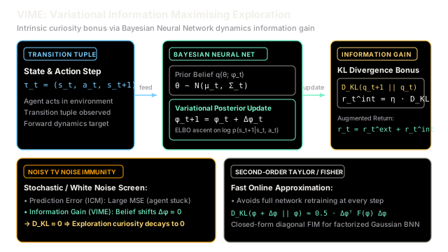
Instead of exploring states with noisy, unpredictable backgrounds, VIME rewards an agent for taking actions that fundamentally improve its internal model of the environment. By measuring the information gain in a Bayesian neural network, curiosity is directed toward learnable dynamics rather than random noise.

VIME computes exploration bonuses from the Bayesian information gain (KL divergence) of environment dynamics rather than raw prediction error.

Why Does This Exist?

In sparse-reward environments, reinforcement learning agents cannot rely on external task feedback to guide early learning. To discover distant goals, agents require intrinsic motivation—an exploration bonus that encourages visiting unfamiliar states.

Early curiosity-based methods, including classic forward dynamics prediction and early variants of Curiosity-Driven Exploration (ICM), compute intrinsic rewards based on prediction error:

r_t^{\mathrm{int}} = \|\hat{s}_{t+1} - s_{t+1}\|_2^2

While effective in deterministic worlds, prediction-error exploration collapses in the presence of stochasticity. This failure is known as the Noisy TV dilemma: an agent facing an inherently random signal (such as a TV flickering static white noise or raindrops falling on water) experiences massive prediction error indefinitely. Hypnotized by unpredictable noise, the agent stays glued to the static screen, accumulating curiosity rewards without making any task progress.

The root problem is that prediction error fails to distinguish between aleatoric uncertainty (inherent, irreducible randomness in the environment) and epistemic uncertainty (uncertainty arising from lack of knowledge about learnable dynamics).

Variational Information Maximising Exploration (VIME), formulated by Houthooft et al. (2016), eliminates this trap by defining curiosity through information gain. Instead of rewarding surprise, VIME rewards the agent for taking actions that actively resolve epistemic uncertainty about the environment's underlying transition mechanics. By maintaining a Bayesian Neural Network (BNN) over dynamics parameters, VIME computes how much observing a transition actually updates its belief distribution. Because pure white noise cannot be compressed into structured dynamics, the agent's posterior distribution stops updating ( $D_{\mathrm{KL}} \to 0$ ), making VIME immune to the Noisy TV trap.

Think of It Like This

The Curious Physicist versus the Coin Flipper

Imagine a physicist conducting experiments in a materials laboratory versus a gambler watching an unbiased coin toss.

When the physicist synthesizes a new superconductor and tests its conductivity near absolute zero, the electrical resistance drops unexpectedly. The physicist checks their instruments and discovers that this single measurement dramatically narrows the probability distribution over plausible physical equations describing the material. Their internal model of physics undergoes massive information gain: before the test, their beliefs were diffuse; after the test, their equations are tightly constrained. The physicist is thrilled and motivated to perform follow-up tests because their foundational knowledge expanded.

Now suppose someone rolls an unbiased 20-sided die repeatedly or leaves a television set on an untuned channel showing snow. A naive observer who measures curiosity purely by "surprise" (prediction error) is permanently captivated: "I guessed the pixel would turn gray, but it turned black! What a huge error!" They stand mesmerized by the screen forever.

The physicist, however, evaluates how much each frame of static updates their fundamental laws of physics. After observing the static for a fraction of a second, their theoretical model of the screen's distribution has stabilized. No single new frame of static alters their physical theories. The information gain is zero ( $D_{\mathrm{KL}} \approx 0$ ). The physicist promptly leaves the room to pursue experiments that actually teach them something new.

Where the analogy stops: A human scientist uses abstract symbolic reasoning to reject noise qualitatively. A deep RL agent using VIME must represent its beliefs over thousands of continuous neural network weights, using variational distributions and second-order Fisher Information approximations to measure whether an experience genuinely improved its dynamics model.

How It Actually Works

Information Gain and Variational Bayesian Dynamics

Let $\xi_t = (s_1, a_1, s_2, a_2, \dots, s_t, a_t)$ denote the history of interaction transitions recorded by the agent up to time step $t$ .

The agent models transition dynamics $p(s_{t+1} \mid s_t, a_t; \theta)$ parameterized by neural network weights $\theta$ . In the Bayesian framework, $\theta$ is a random variable characterized by a probability distribution. Before observing the transition outcome $s_{t+1}$ , the agent possesses a prior belief $p(\theta \mid \xi_t)$ .

Upon observing the subsequent state $s_{t+1}$ , the exact posterior distribution over model weights follows Bayes' rule:

p(\theta \mid \xi_t, s_{t+1}) = \frac{p(s_{t+1} \mid s_t, a_t; \theta) \, p(\theta \mid \xi_t)}{p(s_{t+1} \mid \xi_t)}

The information gain regarding the true dynamics parameters $\Theta$ yielded by observing next state $S_{t+1}$ conditioned on state $s_t$ and action $a_t$ equals the mutual information $I(S_{t+1}; \Theta \mid s_t, a_t)$ :

I(S_{t+1}; \Theta \mid s_t, a_t) = D_{\mathrm{KL}}\Big(p(\theta \mid \xi_t, s_{t+1}) \,\Big\|\, p(\theta \mid \xi_t)\Big)

where $D_{\mathrm{KL}}(\cdot \,\|\, \cdot)$ is the Kullback-Leibler divergence.

Because computing the exact posterior over deep neural network weights is intractable, VIME applies variational inference (specifically mean-field Bayes by Backprop). The intractable posterior is approximated by a factorized Gaussian distribution $q(\theta; \phi)$ :

q(\theta; \phi) = \prod_{i=1}^{|\Theta|} \mathcal{N}\left(\theta_i; \mu_i, \sigma_i^2\right)

where the variational parameters $\phi = \{(\mu_i, \sigma_i)\}_{i=1}^{|\Theta|}$ represent the mean and standard deviation of each individual weight.

At step $t$ , the current variational belief is $q(\theta; \phi_t)$ . When the agent executes action $a_t$ in state $s_t$ and transitions to $s_{t+1}$ , the variational parameters are updated to $\phi_{t+1}$ by optimizing the variational lower bound (ELBO):

\phi_{t+1} = \arg\min_\phi \left\{ D_{\mathrm{KL}}\Big(q(\theta; \phi) \,\Big\|\, q(\theta; \phi_t)\Big) - \mathbb{E}_{q(\theta; \phi)}\big[\log p(s_{t+1} \mid s_t, a_t; \theta)\big] \right\}

The intrinsic exploration bonus $r_t^{\mathrm{int}}$ is set directly proportional to the information gain between the updated posterior and the prior:

r_t^{\mathrm{int}} = \eta \cdot D_{\mathrm{KL}}\Big(q(\theta; \phi_{t+1}) \,\Big\|\, q(\theta; \phi_t)\Big)

where $\eta > 0$ is a curiosity scaling hyperparameter. The augmented reward optimized by the policy algorithm (such as Trust Region Policy Optimization (TRPO) or Proximal Policy Optimization (PPO)) is:

r_t = r_t^{\mathrm{ext}} + r_t^{\mathrm{int}}

Second-Order Fisher Information Approximation

Performing multi-step backpropagation to compute $\phi_{t+1}$ for every single environment transition would cause catastrophic wall-clock training slowdowns. Houthooft et al. accelerate this process by taking a single gradient ascent step on the likelihood and approximating the resulting KL divergence via a second-order Taylor expansion around $\phi_t$ :

D_{\mathrm{KL}}\Big(q(\theta; \phi_t + \Delta \phi) \,\Big\|\, q(\theta; \phi_t)\Big) \approx \frac{1}{2} \Delta \phi^\top F(\phi_t) \Delta \phi

where $F(\phi_t)$ is the Fisher Information Matrix of $q(\theta; \phi_t)$ .

For a diagonal factorized Gaussian distribution, the Fisher Information Matrix is completely decoupled and available in closed form:

F_{\mu_i} = \frac{1}{\sigma_i^2}, \qquad F_{\sigma_i^2} = \frac{1}{2\sigma_i^4}

Taking $\Delta \phi = \alpha \nabla_\phi \mathbb{E}_{q(\theta; \phi_t)}[\log p(s_{t+1} \mid s_t, a_t; \theta)]$ allows the agent to evaluate the exploration bonus in closed form on every environment step without retraining the dynamics network.

Worked numerical example

To trace the mechanism with exact numbers, consider a single dynamics weight parameter $\theta$ with a Gaussian prior belief:

q(\theta; \phi_t) = \mathcal{N}\left(\mu_0 = 1.0, \, \sigma_0^2 = 0.25\right)

The prior precision is $\lambda_0 = \frac{1}{\sigma_0^2} = \frac{1}{0.25} = 4.0$ .

The agent observes transition $(s_t, a_t, s_{t+1})$ . Suppose the likelihood provides parameter evidence with observed value $\hat{\theta}_{\mathrm{obs}} = 1.6$ and observation precision $\lambda_{\mathrm{obs}} = 2.0$ .

1. Bayesian Conjugate Posterior Update

Under Gaussian conjugate updating:

\sigma_{\mathrm{new}}^2 = \frac{1}{\lambda_0 + \lambda_{\mathrm{obs}}} = \frac{1}{4.0 + 2.0} = \frac{1}{6.0} \approx 0.1667

\mu_{\mathrm{new}} = \sigma_{\mathrm{new}}^2 \cdot (\lambda_0 \mu_0 + \lambda_{\mathrm{obs}} \hat{\theta}_{\mathrm{obs}}) = \frac{1}{6.0} \cdot (4.0 \cdot 1.0 + 2.0 \cdot 1.6)

\mu_{\mathrm{new}} = \frac{1}{6.0} \cdot (4.0 + 3.2) = \frac{7.2}{6.0} = 1.2000

2. Analytical Gaussian KL Divergence

The exact Kullback-Leibler divergence from the updated posterior $q_{\mathrm{new}} = \mathcal{N}(\mu_{\mathrm{new}}, \sigma_{\mathrm{new}}^2)$ to the prior $q_{\mathrm{old}} = \mathcal{N}(\mu_0, \sigma_0^2)$ is:

D_{\mathrm{KL}}(q_{\mathrm{new}} \,\|\, q_{\mathrm{old}}) = \frac{1}{2} \left[ \frac{\sigma_{\mathrm{new}}^2}{\sigma_0^2} + \frac{(\mu_0 - \mu_{\mathrm{new}})^2}{\sigma_0^2} - 1 + \ln\left(\frac{\sigma_0^2}{\sigma_{\mathrm{new}}^2}\right) \right]

Evaluating each constituent term:

Variance ratio: $\frac{0.1667}{0.2500} = 0.6667$
Normalized mean displacement: $\frac{(1.0 - 1.2)^2}{0.25} = \frac{(-0.2)^2}{0.25} = \frac{0.04}{0.25} = 0.1600$
Unit offset: $-1.0000$
Log ratio of variances: $\ln\left(\frac{0.25}{0.1667}\right) = \ln(1.50) \approx 0.4055$

Summing the terms inside the brackets:

0.6667 + 0.1600 - 1.0000 + 0.4055 = 0.2322

Multiplying by $0.5$ :

D_{\mathrm{KL}}(q_{\mathrm{new}} \,\|\, q_{\mathrm{old}}) = 0.5 \times 0.2322 = 0.1161

3. Second-Order Fisher Information Comparison

The parameter displacements are:

\Delta \mu = 1.2 - 1.0 = 0.2, \qquad \Delta \sigma^2 = 0.1667 - 0.2500 = -0.0833

The diagonal Fisher Information entries evaluated at the prior are:

F_{\mu} = \frac{1}{\sigma_0^2} = 4.0, \qquad F_{\sigma^2} = \frac{1}{2 \sigma_0^4} = \frac{1}{2 \cdot (0.25)^2} = 8.0

Applying the second-order Taylor expansion:

\frac{1}{2} \left( F_{\mu} (\Delta \mu)^2 + F_{\sigma^2} (\Delta \sigma^2)^2 \right) = \frac{1}{2} \left( 4.0 \cdot 0.04 + 8.0 \cdot 0.00694 \right)

= \frac{1}{2} (0.1600 + 0.0556) = \frac{1}{2} (0.2156) = 0.1078

The second-order Fisher approximation ( $0.1078$ ) closely tracks the exact analytical divergence ( $0.1161$ ) while requiring only single-pass gradient products.

4. Intrinsic Exploration Reward

With curiosity scaling hyperparameter $\eta = 1.0$ :

r_t^{\mathrm{int}} = \eta \cdot D_{\mathrm{KL}}(q_{\mathrm{new}} \,\|\, q_{\mathrm{old}}) = 1.0 \times 0.1161 = 0.1161

This positive bonus is added directly to the agent's reward channel for that transition step.

Code

1import numpy as np2
3
4class VariationalBelief:5    """Represents a diagonal Gaussian variational distribution over parameters.6
7    q(theta; phi) = prod_i N(mu_i, var_i)8    """9
10    def __init__(self, mu: np.ndarray, var: np.ndarray) -> None:11        self.mu = np.asarray(mu, dtype=np.float64)12        self.var = np.asarray(var, dtype=np.float64)13        if np.any(self.var <= 0):14            raise ValueError("Variance components must be strictly positive.")15
16    def kl_divergence(self, prior: "VariationalBelief") -> float:17        """Computes exact analytical KL divergence D_KL(self || prior)."""18        term_var_ratio = self.var / prior.var19        term_mean_diff = (prior.mu - self.mu) ** 2 / prior.var20        term_log_ratio = np.log(prior.var / self.var)21        kl = 0.5 * np.sum(term_var_ratio + term_mean_diff - 1.0 + term_log_ratio)22        return float(kl)23
24    def fisher_approx_kl(self, prior: "VariationalBelief") -> float:25        """Approximates D_KL(self || prior) via second-order Taylor/Fisher expansion."""26        delta_mu = self.mu - prior.mu27        delta_var = self.var - prior.var28        fisher_mu = 1.0 / prior.var29        fisher_var = 1.0 / (2.0 * (prior.var**2))30        approx = 0.5 * np.sum(fisher_mu * (delta_mu**2) + fisher_var * (delta_var**2))31        return float(approx)32
33
34class VIMEExplorationBonus:35    """Computes VIME intrinsic exploration rewards from dynamics information gain."""36
37    def __init__(self, eta: float = 1.0) -> None:38        self.eta = eta39
40    def compute_intrinsic_reward(41        self, prior: VariationalBelief, posterior: VariationalBelief42    ) -> float:43        """Computes r_int = eta * D_KL(posterior || prior)."""44        information_gain = posterior.kl_divergence(prior)45        return float(self.eta * information_gain)46
47    @staticmethod48    def conjugate_gaussian_update(49        prior: VariationalBelief,50        obs_mean: np.ndarray,51        obs_precision: np.ndarray,52    ) -> VariationalBelief:53        """Updates Gaussian prior to posterior using conjugate Gaussian likelihood."""54        prior_precision = 1.0 / prior.var55        post_var = 1.0 / (prior_precision + obs_precision)56        post_mu = post_var * (prior_precision * prior.mu + obs_precision * obs_mean)57        return VariationalBelief(mu=post_mu, var=post_var)58
59
60if __name__ == "__main__":61    np.set_printoptions(precision=4, suppress=True)62
63    # 1. Initialize prior belief q(theta; phi_t) = N(mu=1.0, var=0.25)64    prior = VariationalBelief(mu=np.array([1.0]), var=np.array([0.25]))65
66    # 2. Observe transition evidence (obs_mean=1.6, precision=2.0)67    vime = VIMEExplorationBonus(eta=1.0)68    posterior = vime.conjugate_gaussian_update(69        prior=prior,70        obs_mean=np.array([1.6]),71        obs_precision=np.array([2.0]),72    )73
74    # 3. Compute exact KL divergence and second-order Fisher approximation75    exact_kl = posterior.kl_divergence(prior)76    fisher_kl = posterior.fisher_approx_kl(prior)77    reward_int = vime.compute_intrinsic_reward(prior, posterior)78
79    print(f"Posterior Mean: {posterior.mu[0]:.4f}")80    # -> Posterior Mean: 1.200081
82    print(f"Posterior Variance: {posterior.var[0]:.4f}")83    # -> Posterior Variance: 0.166784
85    print(f"Exact KL Divergence: {exact_kl:.4f}")86    # -> Exact KL Divergence: 0.116187
88    print(f"Fisher Approx KL: {fisher_kl:.4f}")89    # -> Fisher Approx KL: 0.107890
91    print(f"Intrinsic Reward (eta=1.0): {reward_int:.4f}")92    # -> Intrinsic Reward (eta=1.0): 0.116193
94    # Verifications95    assert np.isclose(posterior.mu[0], 1.2000, atol=1e-4)96    assert np.isclose(posterior.var[0], 0.1667, atol=1e-4)97    assert np.isclose(exact_kl, 0.1161, atol=1e-4)98    assert np.isclose(fisher_kl, 0.1078, atol=1e-4)99    assert np.isclose(reward_int, 0.1161, atol=1e-4)100    print("\nVerification Passed: VIME information gain matches analytical bounds.")101    # -> Verification Passed: VIME information gain matches analytical bounds.

Watch Out For

Second-Order Gradient Computational Bottleneck

Computing Hessian-vector products and Fisher Information Matrices for deep neural network parameters introduces a severe computational bottleneck. Even with diagonal approximations, evaluating variational parameter gradients and backward passes for every individual environment interaction can slow down wall-clock RL training by $5\times$ to $10\times$ relative to standard model-free algorithms.

In addition, on high-dimensional inputs such as raw visual observations, doubling network parameters (maintaining explicit mean $\mu$ and log-variance $\rho$ for every connection) produces high-variance Monte Carlo gradients during reparameterization. This instability can cause curiosity bonuses to fluctuate wildly or collapse prematurely.

To keep training stable and computationally tractable:

Compress observations first: Apply VIME over a compact, low-dimensional latent state embedding (e.g., extracted by an inverse dynamics model or autoencoder) rather than raw pixel spaces.
Batch belief updates: Decouple rollout exploration from full BNN parameter updates. Evaluate intrinsic rewards via lightweight gradient steps on current rollouts, while updating the primary BNN dynamics network on mini-batches sampled from a replay buffer.
Normalize intrinsic bonuses: Standardize $r_t^{\mathrm{int}}$ by tracking a running standard deviation, preventing explosive exploration signals during early training phases from overwhelming external task rewards.

The Quick Version

Information Gain over Prediction Error: VIME quantifies curiosity as the reduction in parameter uncertainty ( $D_{\mathrm{KL}}$ between updated posterior and prior BNN beliefs) rather than raw prediction error.
Immunity to the Noisy TV Problem: Irreducible white noise cannot be compressed into structured dynamics updates; the parameter posterior remains stationary ( $\Delta \phi \approx 0$ ), causing the curiosity bonus to drop to zero.
Variational Bayesian Modeling: Approximates the intractable weight posterior using a factorized Gaussian distribution updated through Bayes by Backprop or conjugate updates.
Second-Order Taylor Approximation: Employs the Fisher Information Matrix ( $D_{\mathrm{KL}} \approx \frac{1}{2} \Delta\phi^\top F(\phi) \Delta\phi$ ) to estimate the exploration bonus analytically during online rollouts without retraining the model.