Transfer Learning and Generalization

Why Does This Exist?

Training every new task from a random policy wastes samples. A warehouse robot that already learned to pick boxes should not relearn vision, grasping, and navigation from zero when the warehouse layout changes slightly. Transfer learning reuses the old policy or value function as the starting point for the new task, then fine-tunes it.

Here is the deal: reuse helps only when the tasks share structure. This page covers how transfer works in RL (pretrained initialization plus fine-tuning), how to measure whether it helped, and how to read the generalization gap across a spread of tasks. It does not re-teach supervised transfer, which lives at transfer learning, and it stays distinct from learning-to-learn approaches such as meta-reinforcement learning and MAML in RL, which optimize for adaptability itself.

You need one prerequisite idea first. A Markov decision process (MDP) is the task description: states, actions, transition dynamics, and rewards. A policy $\pi(a \mid s)$ is your rule for picking action $a$ in state $s$. If those terms feel shaky, start with fundamentals of reinforcement learning, then come back.

Think of It Like This

How It Actually Works

The transfer setup

Call the old task $M_{source}$ (the source MDP) and the new one $M_{target}$ (the target MDP). You already hold $\pi_{source}$, a policy trained on the source, possibly with its value function $V_{source}$.

Transfer in deep reinforcement learning usually means one of three moves:

• Policy initialization: copy the weights of $\pi_{source}$ into the new policy, then keep training on $M_{target}$ with your usual algorithm. Early layers (perception, locomotion primitives) are often frozen for a while; later layers adapt first.
• Value initialization: copy $V_{source}$ or $Q_{source}$ so bootstrapping starts from sane estimates instead of zeros. This matters most when rewards are sparse.
• Behavior prior: keep $\pi_{source}$ frozen as a guide (for exploration or as a KL penalty) while a fresh policy learns. Use this when you fear the old weights will be overwritten too fast.

Fine-tuning is just continued training on $M_{target}$ from this head start, usually with a smaller learning rate than the original run.

Three numbers that tell you if transfer helped

Run two agents on $M_{target}$: one from scratch, one fine-tuned. Compare their learning curves with three metrics:

• Jumpstart: the initial gap. That is $J_{tune}(0) - J_{scratch}(0)$, where $J$ is expected return at step $0$ of target training. In our worked example below it is $240 - 20 = 220$.
• Time to threshold and total reward: how many target steps each agent needs to reach a fixed performance bar, plus the area under each curve. Faster crossing with equal final quality is a pure sample saving.
• Asymptotic performance: the final gap once both curves flatten, $J_{tune}(\infty) - J_{scratch}(\infty)$. Here $560 - 520 = 40$.

A transfer can win on jumpstart yet lose asymptotically if the initialization traps the policy in a worse local optimum. Report all three, not just the pretty early curve.

Worked example: from scratch versus fine-tuned

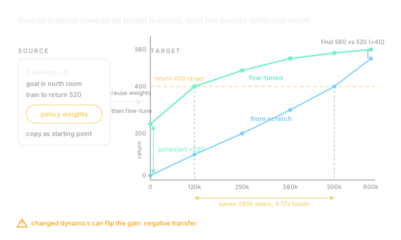
Take a grid navigation task. $M_{source}$ has the goal in the north room; $M_{target}$ moves it behind a new door but keeps the same corridors. Returns are undiscounted episode scores. Both agents train on $M_{target}$ for 600k steps, and we checkpoint them at the same step counts:

• From scratch returns: 20 at 0, 110 at 120k, 200 at 250k, 300 at 380k, 400 at 500k, 520 at 600k.
• Fine-tuned returns: 240 at 0, 400 at 120k, 470 at 250k, 520 at 380k, 545 at 500k, 560 at 600k.

Now compute the three metrics by hand:

• Jumpstart: $240 - 20 = 220$ points of free performance before any target training.
• Time to the 400-point bar: scratch needs 500k steps, fine-tuned needs 120k. Steps saved: $500{,}000 - 120{,}000 = 380{,}000$, which is $380{,}000 / 500{,}000 = 76.0\%$ of the scratch budget. Speedup: $500{,}000 / 120{,}000 \approx 4.17$x.
• Asymptotic gain at 600k: $560 - 520 = 40$ points.

These are the same numbers drawn in the diagram above and recomputed in the code below.

The generalization gap across MDPs

Single-task transfer asks about one pair. Generalization asks about a spread: train on a distribution of MDPs $p(M)$, then test on held-out MDPs from the same spread. The generalization gap is mean test return minus mean train return. A policy can ace its training seeds yet collapse on new layouts, frictions, or goals.

A common way to shrink that gap is domain randomization: train across randomized physics (friction, mass, latency) and visual conditions so one policy covers the whole spread instead of memorizing one simulator. That technique gets its own page; what matters here is the measurement habit. Always report training return and held-out return separately. In our example, a policy averaging 545 on training mazes but 470 on held-out ones has a gap of $545 - 470 = 75$ points, and no transfer claim is complete without that second number. If your target is a robot, the same logic extends to the simulation-to-hardware step, where unmodeled physics acts as one more held-out MDP.

Code

The snippet below recomputes every number quoted above from the two checkpoint series, so you can check the arithmetic instead of trusting it.

1from typing import List2
3
4def transfer_metrics(5    scratch: List[float],6    finetuned: List[float],7    scratch_steps_to_threshold: int,8    finetuned_steps_to_threshold: int,9    train_return: float,10    heldout_return: float,11) -> dict:12    """Compute jumpstart, sample savings, asymptotic gain, and generalization gap."""13    jumpstart = finetuned[0] - scratch[0]14    saved = scratch_steps_to_threshold - finetuned_steps_to_threshold15    pct_saved = 100.0 * saved / scratch_steps_to_threshold16    speedup = scratch_steps_to_threshold / finetuned_steps_to_threshold17    asymptotic_gain = finetuned[-1] - scratch[-1]18    gen_gap = train_return - heldout_return19    return {20        "jumpstart": jumpstart,21        "saved_steps": saved,22        "pct_saved": pct_saved,23        "speedup": speedup,24        "asymptotic_gain": asymptotic_gain,25        "generalization_gap": gen_gap,26    }27
28
29if __name__ == "__main__":30    scratch = [20, 110, 200, 300, 400, 520]31    finetuned = [240, 400, 470, 520, 545, 560]32    m = transfer_metrics(scratch, finetuned, 500_000, 120_000, 545.0, 470.0)33    print(f"jumpstart: {m['jumpstart']:.0f}")34    print(f"saved: {m['saved_steps']:.0f} steps ({m['pct_saved']:.1f}%), speedup: {m['speedup']:.2f}x")35    print(f"asymptotic gain: {m['asymptotic_gain']:.0f}")36    print(f"generalization gap: {m['generalization_gap']:.0f}")

1# -> expected output:2jumpstart: 2203saved: 380000 steps (76.0%), speedup: 4.17x4asymptotic gain: 405generalization gap: 75

Watch Out For

The Quick Version

• Transfer in RL means starting target training from a pretrained policy or value function, then fine-tuning, instead of starting from random weights.
• Judge a transfer with three numbers: jumpstart (here +220), time to a fixed bar (here 120k versus 500k steps, a 380k-step saving at 4.17x), and asymptotic gain (here +40).
• The generalization gap is mean held-out return minus mean training return across an MDP distribution (here 470 versus 545, a 75-point gap), and every transfer claim needs both numbers.
• Negative transfer is real: when source and target dynamics disagree, the old policy can train slower than scratch, so run a short probe before committing the full budget.
• Freezing too much preserves source quirks; unfreeze top-down and reinitialize the value head when reward shapes change.

What to Read Next

• Meta-Reinforcement Learning
• Model-Agnostic Meta-Learning (MAML) in RL
• Deep Reinforcement Learning
• Hierarchical RL