Physics-Informed Scientific ML

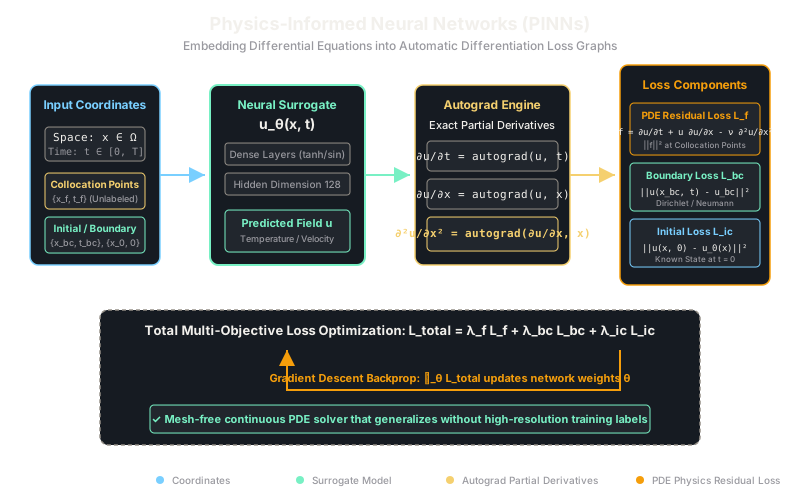
Physics-informed neural networks embed physical laws and differential equations directly into the training loss, turning unlabelled space-time coordinates into physically consistent predictions.

Physics-informed neural networks use automatic differentiation to evaluate differential equation residuals directly in the loss function

Why Does This Exist?

Traditional computational science models physical systems—such as fluid turbulence, heat dissipation, structural deformation, and electromagnetic wave propagation—by solving Partial Differential Equations (PDEs). Numerical methods such as Finite Element Analysis (FEA) and Finite Difference Methods (FDM) require subdividing complex spatial geometries into discrete geometric meshes.

However, numerical solvers face three catastrophic computational bottlenecks:

The Curse of Dimensionality: When solving multi-physics equations in 3D over time ( $3D + 1D$ ), refining mesh spacing by a factor of 10 increases grid points by $10^4 = 10{,}000\times$ , demanding supercomputer compute budgets for high-Reynolds number fluids.
Inverse Problems are Intractable: Inferring unknown physical coefficients (such as thermal conductivity or blood viscosity inside an artery) from sparse sensor measurements requires running thousands of iterative forward PDE simulations inside expensive optimization loops.
Pure Data-Driven Deep Learning Hallucinates: Standard deep neural networks trained purely on input-output sensor data lack physical inductive bias. When evaluated outside the narrow distribution of experimental training runs, they violate fundamental conservation laws—creating artificial energy, allowing negative mass, or violating thermodynamic entropy.

Physics-Informed Neural Networks (PINNs) and scientific machine learning frameworks solve these crises by incorporating continuous differential equations directly into the neural network's optimization objective via automatic differentiation. Rather than needing millions of labeled simulation data points, a PINN acts as a mesh-free continuous solver that trains using unlabelled space-time coordinates.

Before exploring the differential formulation, ensure you understand basic loss formulation in loss-functions, gradient computation in backpropagation, and numerical optimization in gradient-descent.

Think of It Like This

A rookie weather forecaster guided by conservation laws

Imagine two apprentice meteorological analysts hired to predict temperature across an entire mountain valley from just three sparse weather stations.

The pure data-driven analyst connects the three data points with a curvy polynomial line. In between the stations, the curve dips into a bizarre sub-zero frost zone in the middle of a warm summer afternoon. The curve matches the 3 sensors perfectly, but completely violates how heat energy flows.

The physics-informed analyst is given the exact same 3 sensor readings, but is bound by a strict rulebook of thermodynamics: heat cannot spontaneously generate out of nothing, and thermal energy must diffuse outward proportionally to temperature gradients.

Even across empty mountain ridges where zero physical sensors exist, the physics-informed analyst tests their temperature predictions against the heat equation. If a proposed temperature curve predicts heat flowing backwards against a thermal gradient, the rulebook applies an immediate penalty. By continuously adjusting the curve until it satisfies both the 3 sensor readings and the thermal diffusion equations everywhere in the valley, the forecast remains realistic and physically sound.

How It Actually Works

Mesh-Free Continuous Modeling, Automatic Differentiation, and Residual Losses

A Physics-Informed Neural Network parameterizes the unknown continuous field solution $u(x, t)$ of a general nonlinear partial differential equation:

f(x, t) \equiv \frac{\partial u}{\partial t} + \mathcal{N}_x[u] = 0, \quad x \in \Omega, \quad t \in [0, T]

where $\mathcal{N}_x$ is a nonlinear spatial differential operator (such as advection or diffusion), subject to boundary conditions $\mathcal{B}(u) = 0$ on boundary $\partial \Omega$ and initial conditions $u(x, 0) = g(x)$ .

1. The Neural Surrogate Network

A multi-layer perceptron $u_\theta(x, t)$ takes continuous spatial coordinates $x$ and time $t$ as inputs and outputs the predicted physical state (e.g., velocity, pressure, or temperature):

u_\theta: (x, t) \mapsto \hat{u}

Because the inputs are continuous real numbers, the solution is inherently mesh-free: the model can be queried at any arbitrary coordinate $(x^*, t^*)$ without geometric interpolation or grid remeshing.

2. Exact Derivatives via Automatic Differentiation

Instead of approximating derivatives using numerical finite differences ( $\frac{u(x+\Delta x) - u(x)}{\Delta x}$ , which introduces truncation error and requires grid alignment), PINNs compute exact partial derivatives using reverse-mode automatic differentiation:

\frac{\partial u_\theta}{\partial t} = \frac{\partial}{\partial t}\left[ u_\theta(x, t) \right], \quad \frac{\partial u_\theta}{\partial x} = \frac{\partial}{\partial x}\left[ u_\theta(x, t) \right], \quad \frac{\partial^2 u_\theta}{\partial x^2} = \frac{\partial}{\partial x}\left[ \frac{\partial u_\theta}{\partial x} \right]

These partial derivatives are computed with machine precision via the backward computation graph, with respect to the input coordinates rather than network weights.

3. Composite Multi-Objective Loss Formulation

The network weights $\theta$ are optimized by minimizing a composite loss function comprising three distinct penalties:

\mathcal{L}_{\text{total}}(\theta) = \lambda_{\text{res}} \mathcal{L}_{\text{res}}(\theta) + \lambda_{\text{bc}} \mathcal{L}_{\text{bc}}(\theta) + \lambda_{\text{ic}} \mathcal{L}_{\text{ic}}(\theta) + \lambda_{\text{data}} \mathcal{L}_{\text{data}}(\theta)

Where:

PDE Residual Loss ( $\mathcal{L}_{\text{res}}$ ): Evaluated at $N_f$ unlabelled collocation points $\{x_i, t_i\}_{i=1}^{N_f}$ sampled uniformly or adaptively across the domain $\Omega \times [0, T]$ : $\mathcal{L}_{\text{res}}(\theta) = \frac{1}{N_f} \sum_{i=1}^{N_f} \left\| f(x_i, t_i; \theta) \right\|^2$
Boundary Condition Loss ( $\mathcal{L}_{\text{bc}}$ ): Enforces physical constraints along the boundaries $\partial \Omega$ : $\mathcal{L}_{\text{bc}}(\theta) = \frac{1}{N_{\text{bc}}} \sum_{j=1}^{N_{\text{bc}}} \left\| \mathcal{B}(u_\theta(x_j^{\text{bc}}, t_j)) \right\|^2$
Initial Condition Loss ( $\mathcal{L}_{\text{ic}}$ ): Matches the known state at $t = 0$ : $\mathcal{L}_{\text{ic}}(\theta) = \frac{1}{N_{\text{ic}}} \sum_{k=1}^{N_{\text{ic}}} \left\| u_\theta(x_k, 0) - g(x_k) \right\|^2$

When physical parameters are unknown (e.g., fluid viscosity $\nu$ ), they are treated as learnable parameters $\hat{\nu}$ and optimized simultaneously alongside network weights $\theta$ via standard backpropagation, solving complex inverse problems in a single training run.

Worked Example

Let us examine the 1D viscous Burgers' equation, a standard benchmark for nonlinear advection and shock formation:

f(x, t) = \frac{\partial u}{\partial t} + u \frac{\partial u}{\partial x} - \nu \frac{\partial^2 u}{\partial x^2} = 0

Let viscosity be $\nu = 0.01$ . Suppose at a specific unlabelled collocation point $(x_0, t_0) = (0.5, 0.2)$ , the surrogate network currently predicts:

u_\theta(0.5, 0.2) = 0.800

Applying automatic differentiation through the network's input graph yields:

\frac{\partial u}{\partial t} = -0.450, \quad \frac{\partial u}{\partial x} = 0.600, \quad \frac{\partial^2 u}{\partial x^2} = 2.000

Now calculate the PDE residual $f$ :

\text{Advection term: } u \frac{\partial u}{\partial x} = 0.800 \times 0.600 = 0.480

\text{Diffusion term: } \nu \frac{\partial^2 u}{\partial x^2} = 0.01 \times 2.000 = 0.020

f(0.5, 0.2) = \frac{\partial u}{\partial t} + u \frac{\partial u}{\partial x} - \nu \frac{\partial^2 u}{\partial x^2} = -0.450 + 0.480 - 0.020 = 0.010

The squared residual at this point is:

\mathcal{L}_{\text{res}} = (0.010)^2 = 0.0001

Because $f \neq 0$ , the network's current field prediction violates momentum conservation by $0.010$ . The gradient $\nabla_\theta \mathcal{L}_{\text{res}}$ will nudge the network's weights to bring $f(0.5, 0.2) \to 0$ .

Code

The following script implements a minimal PINN in PyTorch that solves the 1D heat equation $\frac{\partial u}{\partial t} - \alpha \frac{\partial^2 u}{\partial x^2} = 0$ using automatic differentiation to compute the physical residual loss:

1import torch2import torch.nn as nn3
4
5class HeatPINN(nn.Module):6    """Surrogate network predicting temperature u(x, t)."""7
8    def __init__(self):9        super().__init__()10        self.net = nn.Sequential(11            nn.Linear(2, 32),12            nn.Tanh(),13            nn.Linear(32, 32),14            nn.Tanh(),15            nn.Linear(32, 1),16        )17
18    def forward(self, x: torch.Tensor, t: torch.Tensor) -> torch.Tensor:19        inputs = torch.cat([x, t], dim=1)20        return self.net(inputs)21
22
23def compute_pde_residual(24    model: nn.Module, x: torch.Tensor, t: torch.Tensor, alpha: float = 0.125) -> torch.Tensor:26    """Compute physical residual: f = du/dt - alpha * (d2u/dx2)."""27    x.requires_grad_(True)28    t.requires_grad_(True)29
30    u = model(x, t)31
32    # First derivatives via autograd33    u_t = torch.autograd.grad(u, t, grad_outputs=torch.ones_like(u), create_graph=True)[0]34    u_x = torch.autograd.grad(u, x, grad_outputs=torch.ones_like(u), create_graph=True)[0]35
36    # Second spatial derivative37    u_xx = torch.autograd.grad(u_x, x, grad_outputs=torch.ones_like(u_x), create_graph=True)[0]38
39    # Physical PDE residual40    residual = u_t - alpha * u_xx41    return residual42
43
44# Seeded demonstration of PDE residual computation45torch.manual_seed(42)46model = HeatPINN()47
48# Collocation points (x in [-1, 1], t in [0, 1])49x_colloc = torch.tensor([[0.5], [-0.2], [0.0]], dtype=torch.float32)50t_colloc = torch.tensor([[0.1], [0.4], [0.8]], dtype=torch.float32)51
52residual = compute_pde_residual(model, x_colloc, t_colloc, alpha=0.1)53pde_loss = torch.mean(residual**2)54
55print(f"Collocation residual values:\n{residual.detach().numpy().round(4)}")56print(f"Mean squared PDE loss: {pde_loss.item():.6f}")57# -> Collocation residual values:58# -> [[ 0.0526]59# ->  [-0.0457]60# ->  [-0.0494]]61# -> Mean squared PDE loss: 0.002434

Watch Out For

Pathological gradient imbalances across multi-objective loss terms

The most common failure mode when training PINNs is gradient stiffness: the gradients originating from the high-frequency PDE residual loss ( $\nabla_\theta \mathcal{L}_{\text{res}}$ ) frequently have orders of magnitude higher variance and conflicting directions compared to the boundary condition gradients ( $\nabla_\theta \mathcal{L}_{\text{bc}}$ ). As a result, standard Adam optimization often gets trapped in trivial local minima (such as predicting $u(x, t) \equiv 0$ everywhere, which satisfies the PDE but completely violates boundary conditions). Always employ dynamic loss balancing algorithms—such as Learning Rate Annealing or GradNorm—to adaptively scale $\lambda_{\text{res}}$ and $\lambda_{\text{bc}}$ during training.

The Quick Version

Physics-Informed Neural Networks (PINNs) solve differential equations mesh-free by taking spatial coordinates $(x, t)$ as inputs.
Exact differential operators are computed using reverse-mode automatic differentiation rather than finite differences.
The training objective combines sparse observation data loss with boundary, initial, and unlabelled PDE residual losses.
Collocation points require zero external labels: the model is supervised purely by whether its derivatives satisfy conservation laws.
Unknown physical parameters (like viscosity or conductivity) can be discovered simultaneously, solving complex inverse problems.