Robot Underactuation and Controllability

A robot can move a joint that has no motor by exploiting coupling with another motion. That does not give it independent control of every acceleration at every instant.

A force on the cart selects a coupled acceleration pair rather than independent cart and pendulum accelerations.

Why Does This Exist?

A cart motor pushes a pendulum's support, yet the pendulum rotates without a motor at its hinge. Underactuation means the available inputs cannot independently specify every generalized acceleration at a state. Controllability asks whether input histories can move the state between desired values over time. Missing instantaneous authority and missing eventual reachability are different questions.

Degrees of freedom counts independent configuration coordinates. A state also includes velocities. Dynamics relates effort to acceleration. This page adds an input map and a passive coordinate; it does not repeat the no-sideways-slip constraint of a wheeled base.

Think of It Like This

Moving a hanging shopping bag by its handle

Move your hand sideways and the bag swings, although you cannot apply a separate turning torque at the flexible handle. Changing hand motion at the right times can build or reduce the swing. Your hand corresponds to the driven cart, the hanging bag to the passive pendulum, and the handle constraint to their coupling. The analogy stops at the bag's flexibility: the worked system is a rigid, fixed-length link with a point mass and no damping.

How It Actually Works

Where do inputs enter the dynamics?

For configuration $q$ , a common mechanical model is

$M(q)\ddot q+c(q,\dot q)+g(q)=B(q)u.$

$M$ is the positive-definite mass matrix, $c$ the velocity-dependent load, $g$ the gravity-balancing load, $u$ the input vector and $B$ its map to generalized forces. Dots mean time derivatives. At a fixed state, possible accelerations are the drift acceleration plus the column space of $M^{-1}B$ . If $B$ has rank below the number of independent coordinates, those accelerations occupy fewer dimensions. Even enough motor channels don't help if their generalized-force directions are dependent. Torque saturation is a separate constraint on input magnitude.

Tedrake's introduction defines underactuation through available acceleration authority. Coupling means a zero entry in $Bu$ does not imply zero acceleration in that coordinate: $M$ needn't be diagonal.

Compute one cart-pole instant

Use a cart on a horizontal rail, with cart mass $m_c=1$ kg. A massless rigid pendulum of length $l=1$ m carries point mass $m_p=1$ kg. The cart coordinate $x$ is positive right; pendulum angle $\theta$ is counterclockwise from vertically downward, positive when the initially downward bob moves right. The bob position is $(x+l\sin\theta,-l\cos\theta)$ in a fixed right/up frame. Input $u$ is horizontal cart force in newtons. Gravity magnitude is $g=9.81$ m/s²; there is no hinge torque, friction or rail limit in this model.

The coupled equations are

(m_c+m_p)\ddot x+m_p l\cos\theta\,\ddot\theta -m_p l\sin\theta\,\dot\theta^2=u,

$l\ddot\theta+\cos\theta\,\ddot x+g\sin\theta=0.$

The second equation is the passive coordinate's constraint on accelerations, not an independently selectable motor command. The MIT cart-pole derivation obtains these equations from kinetic and potential energy.

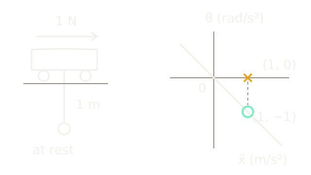
At rest with $\theta=0$ , they reduce numerically to $2\ddot x+\ddot\theta=u$ and $\ddot\theta=-\ddot x$ , with each coefficient carrying its physical units. For $u=1$ N, $\ddot x=1$ m/s² and $\ddot\theta=-1$ rad/s². The bob's instantaneous horizontal acceleration is $\ddot x+l\ddot\theta=0$ : the support initially accelerates beneath it. This is an instant, not the full swing trajectory.

Requesting cart acceleration 1 m/s² while holding angle acceleration zero violates the passive equation at that state. No choice of cart force realizes that pair. The diagram's right panel plots cart acceleration horizontally and angular acceleration vertically, with independent units and 70 drawing units per numerical unit on each axis. Every attainable pair lies on the descending line. The ring at $(1,-1)$ is the 1 N result; the cross at $(1,0)$ is the incompatible request. The left sketch shows the downward starting geometry, not a later deflection. Its push arrow encodes direction only.

How can one input control four state components?

Linearize about the downward rest equilibrium. Let $s=[x,\theta,v,\omega]^T$ , with $v=\dot x$ and $\omega=\dot\theta$ . For the stipulated masses and length, the first-order model is $\dot s=As+Bu$ , where

A=\begin{bmatrix}0&0&1&0\\0&0&0&1\\0&9.81&0&0\\0&-19.62&0&0\end{bmatrix}, \qquad B=\begin{bmatrix}0\\0\\1\\-1\end{bmatrix}.

These numerical matrices assume SI coordinates; entries have the units needed to map the mixed state components. For a four-state continuous linear system, the controllability matrix is $\mathcal C=[B,AB,A^2B,A^3B]$ . Here its columns are

0&1&0&-9.81\\0&-1&0&19.62\\1&0&-9.81&0\\-1&0&19.62&0 \end{bmatrix}.$$ The two independent numerical blocks each have determinant 9.81, and the full matrix has nonzero determinant $-96.2361$. Thus its rank is four. The linearized state can be controlled by a time sequence of forces even though its instantaneous acceleration has only one free input. State evolution exposes directions unavailable at a single instant. This is an unconstrained linear-model result near the equilibrium. It is not a proof that a bounded motor on a finite rail can perform any swing-up or meet a deadline. A horizon that is too short can demand excessive force even when the rank is full. Nonlinear coupling changes with posture; at a horizontal pendulum, the cart acceleration drops out of the passive equation because $\cos\theta=0$. Use trajectory optimization or [model predictive control](/concepts/physical-ai/robot-model-predictive-control) when future momentum and constraints must be coordinated. Direct joint-by-joint tracking works naturally when independent effort authority exists; imposing arbitrary passive-joint references can make the inverse-dynamics problem infeasible. Underactuated mechanisms can save actuators and exploit natural motion, at the cost of more restrictive trajectories and greater dependence on timing and model accuracy. ## Code This offline NumPy example checks both claims: one input restricts instantaneous accelerations, while the local linear model has rank-four controllability. It does not implement a swing-up controller. ```python import numpy as np def acceleration(force: float, theta: float, omega: float) -> np.ndarray: c, s = np.cos(theta), np.sin(theta) mass = np.array([[2.0, c], [c, 1.0]]) rhs = np.array([force + s * omega**2, -9.81 * s]) return np.linalg.solve(mass, rhs) actual = acceleration(1.0, 0.0, 0.0) assert np.allclose(actual, [1.0, -1.0]) assert not np.isclose(1.0 + 0.0, 0.0) # passive equation rejects (1, 0) A = np.array([[0, 0, 1, 0], [0, 0, 0, 1], [0, 9.81, 0, 0], [0, -19.62, 0, 0]], dtype=float) B = np.array([[0.0], [0.0], [1.0], [-1.0]]) C = np.hstack([B, A @ B, A @ A @ B, A @ A @ A @ B]) rank = int(np.linalg.matrix_rank(C)) assert rank == 4 print("accelerations:", actual) print(f"controllability rank={rank}, determinant={np.linalg.det(C):.4f}") ``` Output: `accelerations: [ 1. -1.]` and `controllability rank=4, determinant=-96.2361`. ## Watch Out For <PitfallCard title="A passive joint receives an impossible reference"> An optimizer prescribes independent cart and hinge accelerations, then cannot find a force. Include the passive dynamics as equality constraints. Penalizing tracking error cannot replace a missing actuator; the reference itself may need to change. </PitfallCard> <PitfallCard title="A rank test becomes a promise about hardware"> Full local controllability says nothing about permitted force, rail travel or large-angle reachability on a deadline. Keep the operating point, linearization range and input assumptions with the result. Check constrained nonlinear trajectories before interpreting the local model as a feasible maneuver. </PitfallCard> ## The Quick Version - Underactuation limits instantaneous acceleration authority; controllability concerns motion through time. - Dynamic coupling lets an input accelerate coordinates with no direct actuator. - The downward cart-pole example gives accelerations 1 m/s² and −1 rad/s² from 1 N. - The same example's four-state linearization has rank-four controllability with unconstrained input. - Local controllability does not establish bounded-force swing-up, rail clearance or global reachability.