Seasonality and Trends in Time Series

A shop climbs all year then spikes every December. The climb is the trend, the December spike is seasonality, and mixing them up ruins forecasts.

Twelve months climb from 100 to 122 while December adds 30 and June drops 10, so raw sales mix trend with season

Why Does This Exist?

Daily shop sales look chaotic. One week you sell 100 units, next week 152, then back to 100. If you hand that raw line to a model, it tries to learn two forces at once: the slow climb as your brand grows, and the calendar bumps that return every year. It blends them, so a normal December looks like explosive growth and a normal June looks like collapse.

Split the forces and each becomes easy. The trend tells you where the baseline drifts. Seasonality tells you what December or Monday adds on top. You forecast each on its own, then add them back.

This page teaches the split: what counts as trend, what counts as season, and how to tell which combining rule fits. The full teardown into trend plus season plus leftovers lives in time-series decomposition. Why the split matters for modelling lives in stationarity testing. The model that handles season directly is SARIMA.

Basics first: a time series is values in time order, written $y_t$ for the value at time $t$ . If that notation is new, read time series fundamentals first. Everything below assumes you know why order matters.

Think of It Like This

Walking uphill while your dog loops

You walk steadily uphill. Your dog loops around you in the same wide circle, sniffing the same bushes each lap. A drone tracking only the dog sees a wild zigzag. A drone tracking only you sees a clean climb.

Your path is the trend. The dog loop is seasonality. The leash position you actually observe is the sum of both.

Where it stops: your dog chooses its loops and can change them. Seasonality follows the calendar and repeats at a fixed period. And your hill keeps rising only while business grows. Trends flatten, dog loops do not ask permission.

How It Actually Works

Call the observed value $y_t$ , meaning sales at month $t$ . Call the trend $T_t$ , meaning the baseline if seasons vanished. Call the seasonal offset $S_t$ , meaning what the calendar adds at $t$ . Call the leftover $R_t$ , meaning noise you cannot explain.

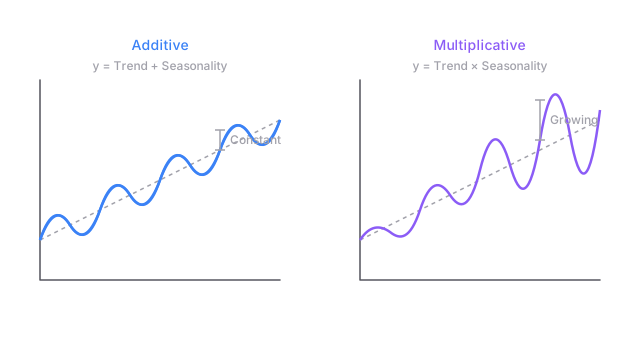
The additive rule says $y_t = T_t + S_t + R_t$ . Use it when December adds about the same units each year. The multiplicative rule says $y_t = T_t \times S_t \times R_t$ . Use it when December adds about the same percent each year, so spikes grow with the brand. Plot yearly peaks: flat height means additive, growing height means multiplicative.

Seasonality needs a fixed period $m$ , meaning the cycle length in steps. Daily data with weekly rhythm has $m = 7$ . Monthly data with yearly rhythm has $m = 12$ . A business boom with no fixed length is a cycle, not a season, and seasonal tools will misfire on it. When in doubt, check autocorrelation: a true season spikes at lags $m$ , $2m$ , $3m$ .

Worked example

Twelve months, trend $T_t = 98 + 2 \times m$ , so month 1 starts at 100 and month 12 reaches 122. Season adds 30 in December and subtracts 10 in June, with 0 leftover.

December: $T_{12} = 98 + 2 \times 12 = 122$ . Then $y_{12} = 122 + 30 + 0 = 152$ .
June: $T_6 = 98 + 2 \times 6 = 110$ . Then $y_6 = 110 - 10 + 0 = 100$ .
The raw jump from June to December is $152 - 100 = 52$ , but the trend only rose $122 - 110 = 12$ . The other 40 is calendar, not growth.

Miss that split and you tell your team demand quadrupled. Split it and you order 30 extra units for December while planning 2 extra per month of real growth.

Code

This snippet recovers yearly means and a fixed seasonal profile with plain lists. Same idea as the diagram, smaller fixture so you can check each step:

1def yearly_means(values: list[float], period: int) -> list[float]:2    """Mean of each full period block."""3    blocks: list[float] = [values[i:i + period] for i in range(0, len(values), period)]4    return [sum(b) / len(b) for b in blocks]5
6
7def seasonal_profile(values: list[float], period: int) -> list[float]:8    """Average offset of each position from its yearly mean."""9    means: list[float] = yearly_means(values, period)10    offsets: list[list[float]] = [[] for _ in range(period)]11    for year, m in enumerate(means):12        for pos in range(period):13            offsets[pos].append(values[year * period + pos] - m)14    return [sum(col) / len(col) for col in offsets]15
16
17sales: list[float] = [100.0, 110.0, 90.0, 120.0, 104.0, 114.0, 94.0, 124.0]18print(yearly_means(sales, 4))  # -> [105.0, 109.0]19print(seasonal_profile(sales, 4))  # -> [-5.0, 5.0, -15.0, 15.0]20print(105.0 + 15.0)  # -> 120.021print(109.0 + 15.0)  # -> 124.0

Yearly means rise 105.0 to 109.0, so the trend gains 4. The fourth-quarter offset repeats at plus 15.0 in both years, so the 120.0 and 124.0 peaks are season plus trend, not a surprise.

Watch Out For

Treating a growing spike as fixed units

You fit the additive rule while peaks grow with the brand. The symptom is a fan shape: residuals look fine early, then December misses by 20, then by 40, always low. The model learned plus 30 units when the truth is plus 25 percent.

Fix it by plotting peak heights against the yearly mean. Flat means additive. Rising together means multiplicative, so take a log or switch models before you trust the intervals.

Calling any wobble seasonal

You fit a 12-month pattern to a business cycle that runs 9 months once and 15 the next. The symptom is a season that never repeats: this January is high, next January is flat, and the forecast confidently picks the wrong one.

Fix it by demanding a calendar reason and a fixed $m$ . Day of week, month of year, hour of day all qualify. A wobble with no fixed $m$ is trend or cycle, so model it there instead of forcing a seasonal term.

The Quick Version

Trend is the slow baseline drift. Seasonality is the fixed-period calendar bump.
Additive means season adds units. Multiplicative means season scales with the level.
A fixed period tied to the calendar is what makes a pattern seasonal.
Twelve months from 100 to 122 plus a December 30 gives 152, not runaway growth.
Check peak heights against the yearly mean to pick additive or multiplicative.
A wobble with no fixed period is a cycle, and seasonal tools will misfire on it.